Clustering

• find pair of vectors with smallest distance
• combine two closest vectors - single genes or average vectors from already assembed subclusters - into a new "subcluster" and remove original objects
• recompute all distances between new "subcluster" and all others

Hierarchical clustering with SUMO

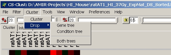
Select Cluster from the main menu:

Cluster

The cluster dialog opens up:

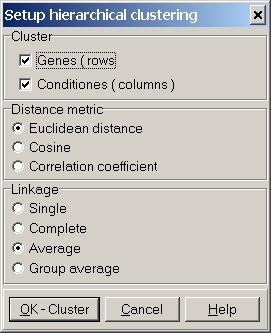
Define the parameters used for clustering:

Cluster

Select to cluster Genes and/or Conditions (=Hybridizations).
Clustering may be performed in one go, or you can first cluster genes, then cluster conditions with different distance metric or linkage.

Distance metric

Several distance metrics may be selected. See below for more details about the metrics.

Linkage

At present three linkage methods may be selected (Group average does not work yet). See below for more details about the metrics.

OK-Cluster button

Run clustering algorithm with specified parameters.

A progress indicator box will show up.

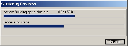
The lower progress indicator bar shows the main processing steps:

• gene distance calculation
• gene clustering
• condition distance calculation
• condition clustering

The upper progress indicator bar shows the progress of each of the (up-to) four steps.

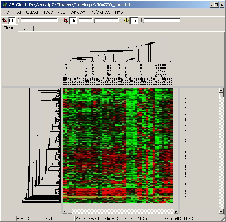
After clustering, the heatmap view will update and show the computed trees:

Distance Metric

• Minkowski distances - measures mainly the absolute similarity of genes
  Typical representatives:
  
  • Eculidean distance
  • Manhattan distance
  • Chebyshev distance
• Gower distance - a variant of Eunclidean distance
• Canberra distance - a variant of Manhattan distance
• Correlation distances - measures mainly the similarity in the shape of the profiles
• Cosine distance - measures the angle between the two vectors
  (very similar to correlation distance)
• "Dot-product" like
• "Jaccard" - binary distance
• "Hamming" - binary distance

Minkowski distance

The Minkowski distance is a generalized distance metric in Euclidean space.

Assume two vectors P,Q with dimension n:


The Minkowski distance of order p is defined as:




Most commonly used are order p= 1,2 and infinite.

Lets look at a very simple example in two dimensional space (n=2):

Manhattan distance (p=1):
Euclidean distance (p=2):
Chebyshev distance (p=infinite):

---

Distances metrices similar to Manhattan distance:

Gower distance

A variant of the Manhatton distance, divided the vector dimension:
      with r = n

Lorentzian distance

Canberra distance

A variant of the Manhattan distance, where each component is normalized to its "length":

Bray-Curtis / Sorensen / Soergel / Czekanowski distance

---

Intersection distance

---

Penrose shape distance

---

Meehl distance

---

Hellinger distance

---

Clark distance

---

Correlation distance

A correlation coefficient is probable more familiar in (linear) regression.

Lets take our two vectors (P,Q), and plot the components (x₁,y₁), (x₂,y₂), (x₃,y₃), ... in a 2-d scatter plot:

If the shape of the data vectors is similar, the data points should be closely scattered around a line (linear regression).
E.g. the two genes (P and Q) are always expressed / regulated in the same way (up / down) for each single hybridisation.

Now we can test whether there is a certain denpendance (=correlation) between the two data vectors:

• Pearson correlation - linear dependance
• Pearson Jackknife - linear dependance, with permutation test
• Spearman correlation - monotonic dependance
• Kendall's Tau correlation - local monotonic dependance

Pearson correlation coefficient

We can test how good the components are lying on a line by computing the Pearson correlation coefficient:


with

The values for r range from -1 ≤ r ≤ 1:

1 =	identical shape of vectors
0 =	no similarity in vector's shape
-1 =	complete opposite shape of the vectors

To transform the Pearson Correlation coefficient to a distance we compute:

d_PC = 1 - r

• 0 = identical shape of vectors
• 1 = no similarity in vector's shape
• 2 = complete opposite shape of the vectors

All three examples view pairs of nicely correlating vectors:

also:

• slope af the regresson line might be different from 1
• absolute values between the vectors might be quite different

The picture illustrates in more details the result of pearson correlation (taken from

Several sets of (x, y) points, with the correlation coefficient of x and y for each set. Note that the correlation reflects the non-linearity and direction of a linear relationship (top row), but not the slope of that relationship (middle), nor many aspects of nonlinear relationships (bottom). N.B.: the figure in the center has a slope of 0 but in that case the correlation coefficient is undefined because the variance of Y is zero.

Kendall's Tau correlation

Kendall Tau correlation coefficient measures even more generalized the association between two datasets.
The non-parametric tests measures the rank correlation, which means the similarity in the order of the data after ranking (=sorting).

Assume two data vectors:

P	4	2	10	6	8
Q	5	20	42	40	3

Lets rank both vectors:

P	4	2	10	6	8
Ranks(P)	2	1	5	3	4
Q	5	20	42	40	3
Ranks(Q)	2	3	5	4	1

Now we analyze the ranks:

	A	B	C	D	E
Ranks(P)	2	1	5	3	4
Ranks(Q)	2	3	5	4	1

Lets analyze each possible pair of data values from vector P and Q.

• Count the pairs where the order of values is identical (concordant pairs, n_c )
• Count the pairs where the order of values is inversed (disconcordant pairs, n_d )

Pair	Data	concordant	dis-concordant
A-B	2 > 1 2 < 3		X
A-C	2 < 5 2 < 5	X
A-D	2 < 3 2 < 4	X
A-E	2 < 4 2 > 1		X
B-C	1 < 5 3 < 5	X
B-D	1 < 3 3 < 4	X
B-E	1 < 4 3 > 1		X
C-D	5 > 3 5 < 4	X
C-E	5 > 4 5 < 1	X
D-E	3 < 4 4 > 1		X
Sum		6	4

4 data pairs have inversed order, thus Kendall tau distance is 4.
Normalized to the number of pairs, Kendall tau distance is 0.4 indicating low association in the rankings.

Similarly we compute the correlation coefficient:

	with	nc=number of concordant pairs
		nd=number of disconcordant pairs)
		n=dimension of data vectors

In the example τ = 0.44, indicating nearly no correlation.

In the present version, SUMO does not take care of ties (= identical numerical value for multiple vector components), as they are not very likely to appear in quasi continuous floating point expression intensities or ratios.

---

Cosinus distance

The Cosinus distance measures the angle between the two vectors P and Q.
The formula and result are very similar to correlation distance.

---

"Dot product"

Minkowski distances are sensitive to the length of the vecotors, correlation distances to the angle between the vectors.

An alternative measure could combine both informations.

The dot product between two vectors is defined as:

Unfortunately, the dotproduct does not fulfill the requirements of a distance metric.
The Dotproduct between two identical vectors is >0, the dotproduct between two orthogonak vectors = 0.


But we can use a modified "dotproduct", where we replace the cosine function with a sine:

---

Binary distances

Special metrices for binary data - a bit unconventional for gene expression data.
For these metrics, data should contain only "1" and "0" vlaues - binary data.
Continuous data vs. binary distance metrices Before clustering with binary distrance, SUMO checks the data:

• All data are binary, i.e. only "1" and "0": data are diretly clustered
• anything else - perform a temporary binarisation.
  Define a threshold value - any data cell >= Threshold will be transformed to "1"
  - all other data cells will be transformed to "0"
  Clustering is now performed with temporary binarized data
  After clustering, the "normal" continuous date are restored.

It may be recommended to permanently transform continuous expression data into binary (1 or 0) values before clustering data when using binary distance.
Use SUMO Main menu | Adjust data | Data transformation | Binarization


Assume two gene / condition vectors x_i and x_j with p elements (in the example p=12 elements):

x_i = ( 1,1,0,1,0,0,1,1,0,1,0,1 )
x_j = ( 1,0,1,1,0,1,1,0,0,0,1,1 )

Now we can count:

n11	number of common existing elements in both vectors ("1" - "1").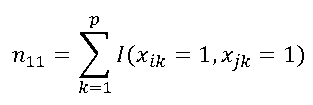 In the example: xi = ( 1,1,0,1,0,0,1,1,0,1,0,1 ) xj = ( 1,0,1,1,0,1,1,0,0,0,1,1 ) n11= 4
n00	number of common missing elements in both vectors ("0" - "0").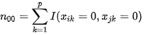 In the example: xi = ( 1,1,0,1,0,0,1,1,0,1,0,1 ) xj = ( 1,0,1,1,0,1,1,0,0,0,1,1) n00= 2
n10	number of elements only exisitng in first vector ("1" - "0") .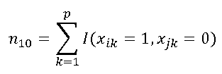 In the example: xi = ( 1,1,0,1,0,0,1,1,0,1,0,1 ) xj = ( 1,0,1,1,0,1,1,0,0,0,1,1 ) n10= 3
n01	number of elements only exisitng in second vector ("0" - "1")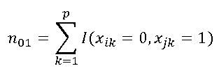 In the example: xi = ( 1,1,0,1,0,0,1,1,0,1,0,1 ) xj = ( 1,0,1,1,0,1,1,0,0,0,1,1 ) n01= 3

With the count numbers n₁₁, n₀₀, n₀₁, n₁₀ we can compute several similarity / distance measures:

---