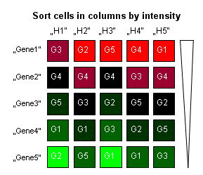
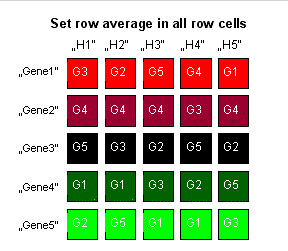
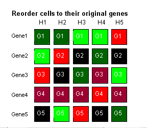
Adjust data

Depending on source of your expression matrix and the planned analyses it might be recommended to adjust data. SUMO offers several basic data adjustment algorithms.


Transpose matrix

Exchange columns with rows (samples with genes).


Truncate data

Sometimes (especially data from single colour arrays) can have negative values. With the Truncate data option you can set all vales below < 0 to e.g. 0.

Select Truncate data | Minimum / Maximum.

This options allows to limit minimum / maximum value of your data to a user defined value.

Sometimes (especially data from single colour arrays) can have negative values. With the Truncate data option you can set all vales below < 0 to e.g. 0.

Select Truncate data | Minimum / Maximum.

A input Dialog pops up:


Enter Minimum / Maximum value.

All data values in your data matrix below Minimum / larger Maximum will be set to Minimum / Maximum.


Conditions

Here you find algorithms to adjust your data column-wise (within single conditions).

Total intensity normalisation

Useful to equilibrate total measured signal from different arrays which may arise from different amounts of labelled RNA/DNA hybridised or from different scanner settings.

The algorithm performs three steps:
  1. Intensity from all features in one hybridisation are added up.
  2. The average of theses sums is calculated:
  3. For each single hybridisation a normalisation factor Average Sum / Hybridisation's sum is calculated
  4. All expression vales (all genes) from each hybridisation are multiplied with the hybridisations normalisation factor.


Total Rank normalisation:

Useful to equilibrate intensity ranges between different hybridisations.

This Algorithm performs three steps:
  1. Sort expression values from a single condition by magnitude
  2. Select the quantile value: Assume you define a quantile value of 30 you will get as normalisation value the 30% value in your sorted data:
    Example you have 10000 genes, the 30% quantile will return you the value at position 3000 from your sorted data set
  3. Divide all values from the respective condition by the respective quantile value
Median normalisation is the special case where Quantile=50.


z-Transformation / Total Variance normalisation

A priori, data in different hybs are most probably differently distributed, due to slight differences in experimental set-up / processing.
I.e. they will have different means (m) and standard deviation (s).
To better analyse data it might be better to transform the data to standard Gaussian distribution, where m=0 and s=1:


Mean variance normalisation

A priori, data in different hybs are most probably differently distributed, due to slight differences in experimental set-up / processing.
I.e. they will have different means (m) and standard deviation (s).
To better analyse data it might be useful to transform the data in such a way they have similar Gaussian like distribution.
In principle very similar to z-transformation. But we do not subtract mean values, and do not force SDev to be one.
In stead SUMO calculates averages and transform all conditions to have all the same means


Quantile normalisation

With this algorithm you force all conditions to have the same distribution of ratios.

The algorithm performs 3 steps:
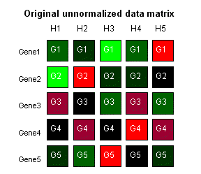
  1. Original expression matrix


  2. Expression values from each hybridisation are sorted (ranked) by their magnitude (memorising their original gene they belong to).


  3. For each of these new "genes", an average expression value from the sorted hybridisations is calculated. This average will replace the individual expression values in all "hybs" for the specific "gene".


  4. The new "quantile normalised" expression values are placed back into the original expression matrix to their corresponding genes.


Due to the time consuming sorting of the expression values, quantile normalisation requires some time especially with large expression matrices.
E.g. ~10s for 45000 genes X 150 conditions on a Pentium4 Dual Core 3.2 GHz.

For details about the method see
Bolstad, B. M., Irizarry R. A., Astrand, M, and Speed, T. P. (2003)
A Comparison of Normalization Methods for High Density Oligonucleotide Array Data Based on Bias and Variance.
Bioinformatics 19,2,pp 185-193
especially cited unpublished manuscript
Bolstad, B (2001) Probe Level Quantile Normalization for High Density Oligonucleotide Array Data




Total rank centering

Useful to equilibrate total measured signal from different arrays which may arise from different amounts of labelled RNA/DNA hybridised or from different scanner settings.

The algorithm performs three steps:
  1. Values from all features in one hybridisation are sorted by magnitude.
  2. The value at the specified percentile is used as centering value.
  3. From all expression values (all genes) from each hybridisation the computed value is subtracted.
This function should be used when log-values (e.g. ct-values from RT-PCR) are used insted of total rankl normalization.


Control normalisation

The previous normalization procedures assume a quasi-Gaussian like random distribution of intensities / ratios.
In case this basic-asumption might not true (non-genome wide datasets, strong directional regulation of a large part of the dataset, pathway specific datasets ...) the previous normalization schemes might not adeqately adjust your data.
Instead, it may be recommended to use well selected contol genes / spike-in controls for normalisation.

For all methods, you have to define:
- gene annotation colum containing control's names
- set of control names

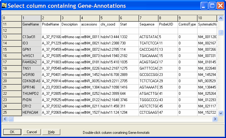
A data prewiew (first view hundred data rows from the presently loaded data matrix) opens up:
Dobule-click the data column which contains the feature information on which the the refernece features shall be defined (e.g. gene name), or click the column then click OK-button.

An Input-dialog opens up:

Define the feature name(s) which shall be used as normalisation references.
You may use multiple search keys, divided by SPACES (which implies, you can search for feature names containing spaces !!).
SUMO will search for "contained" matches, non case sensitive.
E.g.: define "hprt vegf" will present HPRT1, VEGFA,VEGFB, VEGFR

SUMO computes mean/median/regression parameter from the matching controls and performs the specific normalization/centering.

Normalization (division by average) should be applied to "linear" values (e.g. fluorescent intensity as measured by the scanner).

Centering should be applied to log values (e.g. ct-Values from RT-PCR).


Normalisation / Centering with Mean / Median

- SUMO computes Mean / Median for each condition.
- Each data value within a conditon will be divided / subtracted the respective conditions's Mean / Median
This operation will remove the information about data magnitues and generate data centerd around 1 (normalisation) or 0 (centering).


Normalisation / Centering to common Mean / Median

- SUMO computes Mean / Median for each condition
- Average from these Means / Medians is computed
- Normalisation Factor / Minued is computed in such a way, that after normalisation contorl-Means / -Medians in all hybs have the same value.
- Each data value within a conditon will be divided / subtracted by the respective Factor / Minuend.
This operation will only slightly modify the overall data magnitude.


Genes

Here you find algorithms to adjust your data row-wise (within single genes)

Normalisation values may be computed as - arithmetic means (intensities, log ratios) - geometric means (ratios data) - medians (robust outlinier independant)
Depending on data one should perform - normalisation for intensity data (divide individual data by mean) - centering for log data (subtract mean from individual data)

Virtual pool normalisation

The algorithm calculates the mean from all selected conditons within a single gene.
Then each original expression value is divided by this Mean.

For single-colour expression data (fluorescent intensity data) this corresponds to generation of ratio data using a "virtual pool" as reference.


Hybridisation normalisation

For each individual gene, use specific reference samples (controls) to normalize (all) other samples.

You define two groups:
The algorithm normalizes:

  Each single gene from Group 1 normalzed with Average (Group 2)

Of course, you can perform multiple normalisations with respective subsets, e.g.:

Ctrl1Sample1a Sample1a Sample1cCtrl2Sample2a Sample2b Sample2c....

Here you could first normalise all Sample1 / Ctrl1 than Sample2 / Ctrl2 ...

A selection dialog pops-up:


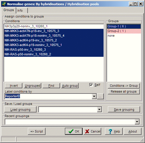
Assign hybridisations to the respective groups as usual.

By default the SELF checkbox is activated. This means, that the reference hybridisation(s) are normalised too.
This will guarantee, that Controls will have a similar data space like the nomalized samples.


ComBat

In complex experiments where data from different sources (e.g. data profiled with the same platform but in different places, or using different slide/chemical batches, version of preprocessing protocols, ....) you might expect/observe overall differences between the respective groups of samples => batch effect.

Simple standard normalisation procedures might not compensate for these batch effects.

ComBat is a specifically designed method to take care of these batch effects.
It tries to estimate the systematic differences between the batches and remove them while preserving the biological question.

For more details about Combat see the publication or visit the ComBat home page.

SUMO does not implement its own ComBat procedure but wraps the R-Package SVM.

Select: Main menu | Adjust | Data | Normalize conditions | Batch compensation | ComBat

The group selection dialog opens up.

Define:
- Number of groups = number of batches in your loaded data set.
- Assign samples (hybridisations) to respective groups

Click OK or Run button to execute ComBat.

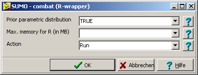
A parameter dialog opens up:


SUMO performs:
- write data for ComBat as tab delimited text files
- generate and write r-script
- Spawn a R-sessions, executing the just generated R-script.
- Wait until R has finalized (may take a while)
- Read transformed data back

NB: Requirements - recommendations

In case of any problems, see the intermediate files created by SUMO in your MS-Windows temp folder (e.g. c:\user\uxerxy\AppData\Local\temp\sumo_combat_....txt).

Pre-Requisites:


VST,Rlog2 - Transformation

One problem in statistical analysis may be that variance within a gene row may depend on signal strength.
On spotted arrays you might expect high variance of lowly expressed genes,
With RNA-Seq data you may observe also high variance with highly expressed genes

The very simple log transformation of measured intensity/count values would mainly reduce the variance in highly epressed genes but even increase the variance in lowly expressed genes.

Variance stabilizing transformations will try to equlibrate the variance in all features independant of signal strength.

As a logical consequences expression differences will also be stabilized.
Thus class tests with rlog/vst-tranformed data may show "stabliized" differential expression, which might be different compared to raw data.
rlog/vst are mainly targeted for applications where the magnitude of differntial expresson (e.g. hierarcical clsutering) is not essential.

vst and rlog2 are two variants of VST's.

SUMO does not implement its own "vst" or "rlog2" procedures but wraps the R-Package DESEQ2 which contains both.


For more details about DESEQ2 (and thus vst and rlog2) see
documentaion for DESEQ2


Select: Main menu | Adjust | Data | Normalize conditions | vst / rlog2

The group selection dialog opens up.

Typically you would assign all samples to one group and apply the procedure to all samples.
But there might be reasons to perform several rounds of transformation using certain (even overlapping) subsets of your samples.

Click OK or Run button to execute vst / rlog2 transformation.


SUMO performs:
- write data as tab delimited text files
- generate and write r-script
- Spawn a R-sessions, executing the just generated R-script.
- Wait until R has finalized (may take a while)
- Read transformed data back

NB:

In case of any problems, see the intermediate files created by SUMO in your MS-Windows temp folder.
(e.g. "c:\user\uxerxy\AppData\Local\temp\sumo_vst_....txt" or "c:\user\uxerxy\AppData\Local\temp\sumo_rlog2_....txt".

Pre-Requisites:


DESeq2

One problem in statistical analysis of RNA-Seq data may be that variance within a gene row may depend on signal strength.
Especially for very low but also for very highly abundant genes variance may be come large, and thus 2-class test may suffer from such high variances.

A specific method may be applied to accomodate for this problem
DESeq2 applies a linear model to reduce variances in the groups of a two class test.
SUMO does not implement its own "DESeq2" procedure but wraps the R-Package DESeq2.


For more details about DESEQ2 see
documentaion for DESEQ2


Select: Main menu | Adjust | Data | Normalize conditions | DESeq2

The group selection dialog opens up.

Assign all required samples to the two groups.

Click OK or Run button to execute DESeq2.


SUMO performs:

NB:

In case of any problems, see the intermediate files created by SUMO in your MS-Windows temp folder.
(e.g. "c:\user\uxerxy\AppData\Local\temp\sumo_dese2_....txt".

Pre-Requisites:


z-Transformation

A priori, data in different genes may be regulated witin a different data range.
E.g. Gene123 is regulated between -1 and +1.
Gene1070 between +4 and +8.
I.e. they will have different means (m) and standard deviation (s).
To better analyse data it might be helpful to transform the data to a similar (same) data range.

z-Transformation

Assuming you data are Gaussian distributed, it may be helpful to transform the data in each gene, that data for each individual gene have standard Gaussian distribution, where Mean m=0 and standard deviation s=1:


z-Transformation (Median, MAD)

Often your data are not nicely normal distributed, but you find a few population "outlier".
Such outliers might disturb coumputation of mean and SDev (e.g. data series 10,1,0.5,1.3,1.2,1)
For such cases it might be better to use a more robust method.
Instead of mean we use the MEDIAN, in stead of standard deviation we use Median Absolute Deviation (MAD).


z-Transformation ( Min,(Max-Min)/2 )

For some analyses it may be helpful to transform the data range from each individual gene to the intervaL 0..1.
So we search Minimum and Maximum value and transform:


Data transformation

Here you find algorithms to numerical transform your data.

Log2 transformation

All data will be transformed into the respective log2 value.
E.g. 1=>0, 2=>1, 4=>2,8=>3, ...
0.5=>-1, 0.25=>2, 0.125=>-3, ....

NB:
"0" or negative values can not be Log2 transformed (mathematically impossible).
These numbers are replaced by 1E-45 (about the smallest single precision number the program can handle).
Thus, it is not recommended to log2 transform datasets which contain negative numbers.
Use the Truncate function (see above) to remove e.g. negative intensity data.


Log10 to Log2 transformation

Some image analysis programs (e.g Agilent's feature extraction) export two-color ratios as log10 values.
For convenience it may be useful to convert the Log10 ratio values into Log2 values.


Exp2 transformation

Compute the power fuction with base 2 of your data.
I.e. transform log2 data into ratios.


Ratio to "Intensity"

Generate fake intensity date from ratio datio, by multiplying the ratios with a fixed user defineable factor.


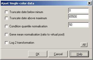
Single colour data adjustment

Here you will find a collection of useful data adjustment functions for pre-normalised (single image normalisation) intensity data.

A Dialog pops up:


Check any of the available options and set corresponding numerical parameters.
If you want to run all options click the All button.


Arithmetic operations

Here you can find some basic arithmetic operations.


Change sign

Simply change sign of data values (e.g 1 => -1).
Useful when working with two-colour DNA micro-array data where direct and dye-swap hybridisations are combined.


Back-up data

When testing the effect of different combinations of data adjustment algorithms it is desireable to work with a common original (or intermediate) data set. Instead of always reloading (and performing the same initial steps) you can "back-up" the working data set (expression matrix and annotations).
Now you can modify the working set any way you want. If you don't like the final result, simply restore a previously created back-up and try other procedures.

E.g. Load data and create initial backup. Now pre-filter (e.g. impute NAN values, remove lines with too low average intensities) and create pre-filter backup.
Now explore the basic normalization routines, always reusing the pre-filter back-up.....

All back-up data sets are stored in a SUMO analysis file.


Back-Up

Create a back-up of the presently loaded working data set - expression data as well as condition and gene annotations.
Each back-up is a one-to-one copy of the loaded data-set and thus will consume mentionable amounts of main memory.
When creating a back-up SUMO asks for a name.


Restore

Restore a previously created backup.
The working data set is removed (including any meanwhile performed filtering, normalisation ... operations) and the data from the selected back-up are restored.
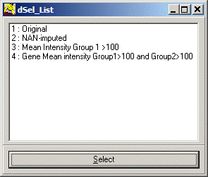
A selection dialog opens up:

Select and double-click the back-up to be restored (or select and click Select button).


Delete

Each single back-up consumes mentionable amounts of main memory. Thus it may be useful to delete no longer required backups from memory to free main memory for statistical analyses within SUMO.
The selection dialog (see above pops-up).
Select the back-up which shall be deleted.


Replica averaging


On many mirco-array platforms / detection systems, features are represented in replicates (identical target / sequence) or multiple features are targeting the same objects/"gene". (multiple target sequences, but the same gene.
A special case of such replication are exon arrays, where for (nearly) each single exon of a gene a feauture is found on the array.

You could analyze the data and hope, that all replicates for the same genen pass your statistical tests and show up together.
You could also compute averages (or other derivatives) from all replicates for a single gene/object and analyze only the averages.

SUMO allows to compute the "averages" according to
  • Arithmetic mean - sensible to outliers (bad or missing features), use for linear/log transformed data
  • Geometric mean - use for ratios
  • Median - not sensible to outliers (if there are clearly more mainstream vs. outliers)
    (median is the special 50% case from percentile)
  • percentile - you define the level. Not sensible to outliers.

  • Replica CV - based on arithmetic mean.
  • Replica CV - based on median mean.
  • Replica coefficient of quartile deviation.

  • Replica count

After replica analysis, the original data values are lost and replaced by the derived data.
Obviously, the number of rows wil be reduced.

In any case you have to define the data column which contains the feature annotation where replicates shall be searched.
A data prewiew (first view hundred data rows from the presently loaded data matrix) opens up:


Double-click the data column which contains the feature information on which the reference features shall be defined (e.g. gene name), or click the column then click OK-button.


Coeffcient of variaton from replicas

Sometimes it might be useful to estmate the variance in your replicated data.
I.e. try to find those genes with high variance between the replicates of all or a subset of your samples.
E.g. find genes where averages from exons have high variances => differntial splicing ??
SUMO allows to compute the coefficient of variation:

         
        cv = ( 1 + 1/4n ) * s / m        

with:
s=sample standard deviation,
m=sample mean, n=sample size
more details

applying as mean:
  • arithmetic mean
  • median
Alternatively - recommended if interval data (i.e. negative and positive numbers) are used - the Coefficient of Quartile Deviation (CQD)could be computed:

         
        CQD = ( Q3 - Q1 ) / (Q3 + Q1 )        

with:
Q1=value of first quartiles, value of (n+1)/4th item
Q3=value of third quartile: value of (3*(n+1))/4th item
more details


If you selected percentile, an Input-dialog opens up. Define the percentile level (between 0-100).

SUMO performs the steps
  • Search unique feature annotations
  • Group features with same annotation
  • Compute average
  • Reorganize data
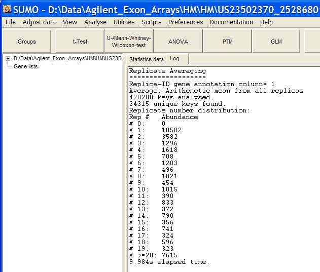
In the Log-tag, a brief summay about replica averaging is shown:


Replica count

In some application (e.g. library screening applications), it may be helpful to count the number of replicated genes (features) where a certain signal level is reached.
E.g. in Crispr/Cas screens, multiple guide sequences for the same gene are used.
Genes where all or many of the guides are found in the sample may be most interesting.

SUMO counts the number of replicates for one feature(gene) where the Intensity (count) is within the user defined threshold.
.
An Input dialog opens up.
Define Low and High counting threshold.

E.g. define Low=10; high=1000: Only replicates with intensities between 10 and 1000 are counted.
Assume replicate numbers (8,123,34,1209,3400,65,312,12,819,1) will result in replica count 6 (out of 10).

To omit low or high threshold, just leave the respective field in the dialog empty.
(Technically: the empty field value is replaced by a very large negative/positive number: +/-9.9E34).

SUMO rebuilds the matrix.
  • Only non-redundant gene (feature) names are left.
  • Intensities are replaced by the respective replica counts.