SUMO - NGS utilities
Here you may find a few functions to perform basic operation with SAM, BED, ... files
| SAM filter | Filter SAM files by Flag, Start and length of reference sequence, Q-value |
| SAM => Population map | Generate a map of sequence bins hit by sequences
from multiple SAM files.
|
| BED tools | A set of tools to work with BED like genomic ranges objects lists |
- View: View (multiple) BED files as line graphs.
- Features to Bumps: Combine closely neghbouring BED objects to a wider "Bump"
- 1/2 class test: find genomic regions hit by multiple BED files, respetively
differentially hit by two different groups of BED files.
- Annotate: Annotate BED-format like files with genomic features.
|
| SAM tools |
A set of tools to work with SAM/BAM files |
- QC: Generate some diagnostic data / plots from SAM/BAM file.
|
Filter SAM
In certain screening applications (Crisp/Cas transfection, LAM PCR, ...) NGS sequencing may be applied to identify target products.
Quality information as well as soft clipping information from genome mappers (e.g. Bowtie2) may be used to skip unwanted features.
SUMO can filter SAM files by:
| SAM flag | Value=0 or 16. Only unique forwared or reverse complemented sequences |
| Sequence start min/max | Range for Length of 5'-sequence not matching to reference.
The SAM's CIGAR is evaluated. Left- as well as right soft-clipped sequences are used to measure
5'-/3'-non reference sequence parts and resulting matching sequence length.
The non matching sequencs may correspond to adapters, parts of the transfection vectors, .... |
| Min match length | Minimum length of sequence matching to reference. |
| Q-value | The Quality value (p-value) of the sequence alignment |
| Map resolution | SUMO may generate a low reolution population map / coverage graph for the whole referenve (genome).
Define a resolution (binsize) for these graphs.
Resolution should be ~1 MegaBP. |
| Type of output | Define the otuput SUMO shall generate:
- s : filtered SAM file (default).
- b : filtered BED file. More compact but no sequences.
- c : coverage plot for each individual SAM input file
- h : histograms for size distributon 5'-/3'-soft clippend / length for each individual SAM file
- h : low resolution population map
define any combination of the respective characters.
E.g. "sm" to generate filtered SAM and Population map. |
Additionally, SUMO automatically generates integrated Coverage and Size Distribution plots from all samples.
Selece Main menu | Utilities | NGS | Filre SAM
A parameter dialog open up:
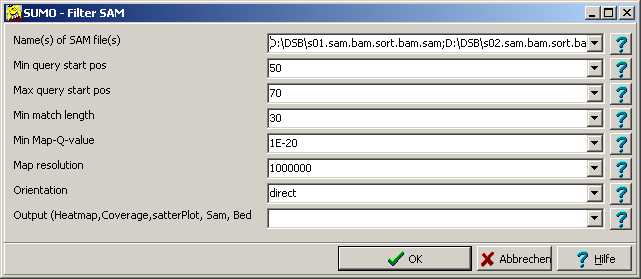
Fill in all parameters accordingly.
Drag one - or multiple - SAM files from Windows' explorer into the Name of SAM files Edit field,
double click the edit field or click the "..." button to open a file selection dialog.
SUMO generates an overall report:
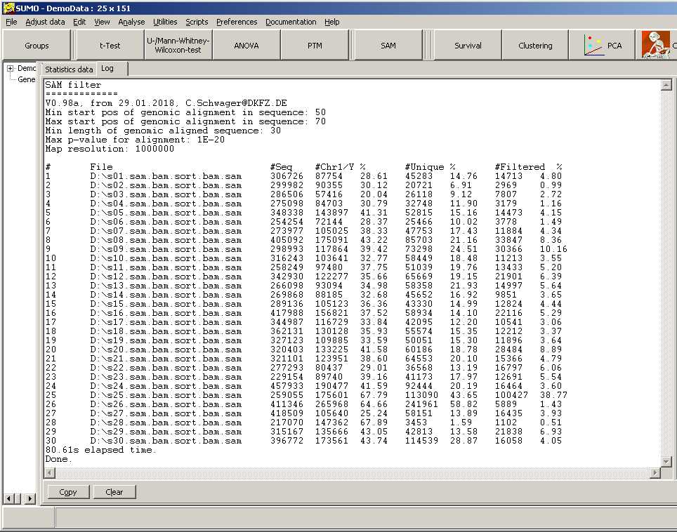
For each sample (SAM file) is shown:
- total number of analyzed sequences
- number of sequences matching to any of the chromosomes
- number of sequences with a single unique match to the genome
- number of sequences passing the filter
Additonal graphs may show:
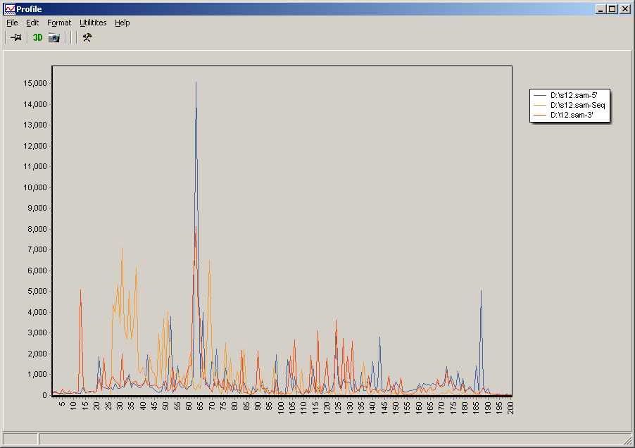
Histograms for each samples, showing length distribution of
- 5'-soft clipped sequence part (i.e. 5'-Linker/adapters not matching to the reference genome (blue).
In the example a maximums appears ~65bp, corresponding to the expected adapter length.
A second maximum around 150bp may indicate constructs with a duplicated adpater.
- Length of sequence homologous to the reference genome (orange).
Large number of very short inserts (25-60)
This graph starts at 25bp - conforming to the lower sequence length threshold defined in the parameter dialog.
- 3'-soft clipped sequence part, not matching to the reference (red).
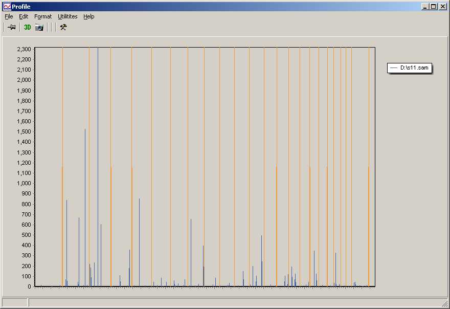
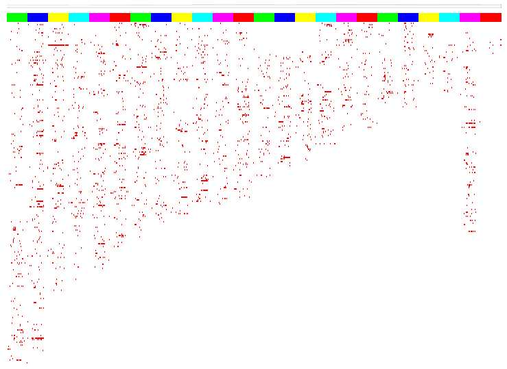
Coverage plot for each sample.
Orange indicates boundaries between chromomes (1-23,x,y).
Blue indicate how often a certain region was hit by the sequences within the respective BAM file.
In the example a resolution of 1000000bp was chosen to generate a coarse overview.
In the example (detection of DSB-sites) the graph indicates very few detected sites accross the genome in an individual sample.
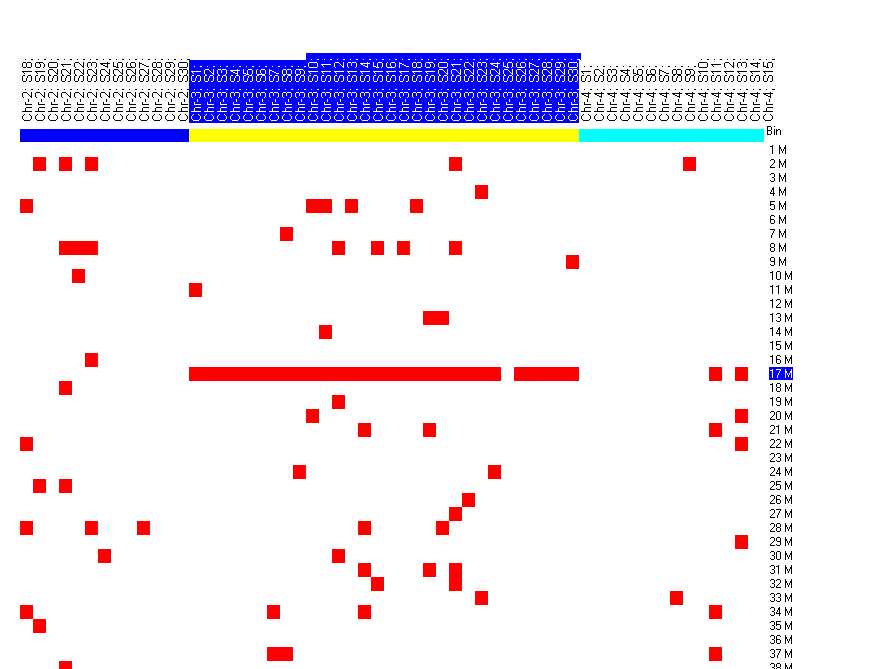
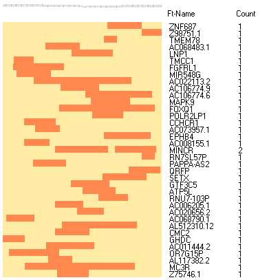
"Population map"
A heatmap like graph shows the distribution of filtered sequences for all samples accross the human genome.
Data columns are grouped by chromosome, to easily recognize conserved patterns between samples.
The colored boxes on top of the heatmap indicate the chromosomes.
Rows represent 1 Mega-BP bins.
In the example, it is easy to see that on chromosome 3 (first yellow box) there is a higly conserved region around 17 M-BPs.
Especially if you zoom into the region:
SAM to population map
BED-tools
A set of tools to work with BED like genomic ranges object lists.
- View: View (multiple) BED files as line graphs.
- Features to Bumps: Combine closely neghbouring BED objects to a wider "Bump"
- 1/2 class test: find genomic regions hit by multiple BED files, respetively
differentiall hit by two different groups of BED files.
- Annotate: Annotate BED-format like files with genomic features.
After alingment (mapping) of sequences to a reference genome, sequence reads are often summarized into genomc intervals (e.g. ChipSeq binding sites, ...).
BED files are simpe lists of these genomic intervals and additional information.
BED file structure:
- ASCII text file with one object per line.
- Each line contains several tab delimited data fields
- 1. field: chrom - name of the chromosome or scaffold.
Any valid seq_region_name can be used,
and chromosome names can be given with or without the 'chr' prefix.
REQUIRED
- 2. field: chromStart - Start position of the feature in standard chromosomal coordinates
(i.e. first base is 0).
REQUIRED
- 3. field: chromEnd - End position of the feature in standard chromosomal coordinates
REQUIRED
- all other fields are optional:
- 4. name - Label of the feature
- 5. score - A score for the particular feature between 0 and 1000 (e.g. count or p-value
- 6. strand - defined as + (forward) or - (reverse)
- and others
A BED file typically looks like:
chr1  213941196  213942363  Pos1  13  +
chr1  213942363  213943530  Pos2  14  +
chr2  158364697  158365864  Neg1  35  -
chr2  158365864  158367031  Pos1  17  +
chr3  127479365  127480532  Pos1   8  +
chr3  127480532  127481699  Neg2  12  -
...
See a more detailed description of BED files and variants.
At present SUMO supports:
- 1. Field: only Chromosome ID: chr1..chr22,chX,chrY,1..22,x,y (non-case sensitive)
- Empty lines / comment lines (starting with #) are ignored
- in some tools, order of fields may be specified (e.g. Start/Stop/Chrom-ID/Score/Strand
BEDPE file Structure
A BED like file containing basic information for both sequecces of Mate pairs form Paired-End sequecing.
- ASCII text file with one object per line.
- Each line contains several tab delimited data fields
- 1. field: Name of the chromosome or scaffold.
Any valid seq_region_name can be used,
and chromosome names can be given with or without the 'chr' prefix.
- 2. field: Start position of the feature in standard chromosomal coordinates for Mate1
- 3. field: End position for Mate1
- 4. field: Name of the chromosome or scaffold for Mate2.
- 5. field: Start position for Mate2
- 6. field: End position for Mate2
- 7. field: Name of the Mate pair
- 8. field: Score
- other fields are optional:
A BED file typically looks like:
10          79359547    79359698    10          79359718    79359869    ST-E00210:236:HYJJ2CCXY:6:1101:3833:1555	44	+	-
KI270438.1	  110047	  110196	KI270438.1	  110098	  110249	ST-E00210:236:HYJJ2CCXY:6:1101:3853:1555	 1	+	-
.	                -1	      -1	.                 -1	      -1	ST-E00210:236:HYJJ2CCXY:6:1101:3975:1555	 0	.	.
14        	89566311	89566461	15	        89566427	89566578	ST-E00210:236:HYJJ2CCXY:6:1101:4239:1555	44	+	-
...
BED-tools - View
A basic tool to visualize content of BED,BEDPE,SAM,BAM file(s) on genomic scale as line graphs:
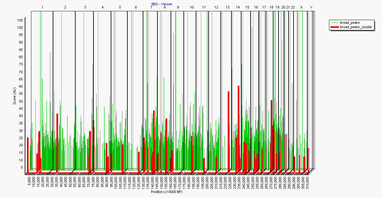
The graph illustrates two BED files (here in 3D projection:
- Green-Line : ChipSeq peaks created with Macs2
- Red-line : Clusters of closely neighbouring Macs2 peaks, generated with SUMO (see below)
Chromosomes boundaries are indicated by black dividers, centromers by gray dividers.
Depending on the pre-selected resolution ( here: 10000 BP) x-axes will be scaled.
You may customize the data view applying ProfileViewers options (e.g. Point-/Bar-/Line-Series, color withth, Zoom, ...).
You may use apply ProfileViewers DSP functions to transform the data (Smooth, BIN, NOrmalize, Log-transform, Segment, ...).
From SUMO's main menu select Main menu | Utilities | NGS | BED: View
A parameter dialog opens up:
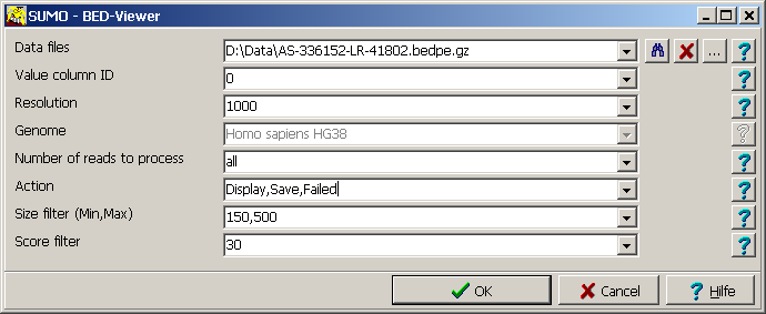
| Data files | Supply a single or a semi-colon separated list of data files.
Click the "..." button to open a file system browser and select desired files.
More easyly: drag one or multiple files from Windows Explorer into the BED viewer dialog.
Newly dropped files are added to the list of already selected files.
To clear the list, click the "X" button.
To preview the (first) file from the selection list click the "binoculars" button.
At present SUMOsupports the file formats:
- BED, file extension "*.bed"
- GZip compressed BED, file extension "*.bed.gz"
- BEDPE file extension "*.bedpe"
- GZip compressed BEDPE, file extension "*.bedpe.gz"
- SAM, file extension "*.sam"
- GZip compressed SAM, file extension "*.sam.gz"
- BAM, file extension "*.bam"
(Only for files with SAM header << 65 KBytes (e.g Genomic alignments).
SUMO tries to parse the repsective filetypes depending on the file extension.
Thus, striclty stick to the expected extensions.
|
| Value column ID | The data column within the BED file containing the value which shall be
displayed on the Y-axes.
Define "0" to just count the coverage.
|
| Resolution | SUMO averages neighbouring BED objects into bins with given size.
In the example bin size (=Resolution) of 10000 BP was selected, resultng in a line graph with 300,000 data points.
You may go down to 100 BP resolution (at least for single BED files) but response time for graphs with ~30 million
will be low.
|
| Genome | At present, only Human genome HG38 is supported (overall size/chromosome dividers).
|
| Reads to process | Often one can reacognize te underlying datastructure when analyzing only a small part of the data (e.g. 10Milion reads).
Define "all" to process the complete data file.
|
| Action | Waht to do with the result data:
Display - Show only th graph.
Save - Save a "Coverage file".
(A tab delimited text file: Start TAB Stop TAB Count)
Failed - A BEDPE file for mates not passing the defined filter (only for BEDPE)
Or any combination of the three.
|
| Chromosome-filter |
Entries with "invalid" chromomes id (i.e. something else thean "1".."22","X","y",MT) are always skipped (and entered to the failed BEDPE).
|
| Pair-filter |
BEDPE entries where Mates are located to different chromosomes are always skipped (and entered to the failed BEDPE).
|
| Size filter |
Filter BEDPE entries an the target sequence region they span (i.e. Start-Mate1 - Stop-Mate2)
Define "Min,Max". BEDPE entries < Min or > Max will be skipped (and entered to the failed BEDPE).
|
| Score filter |
Filter BEDPE entries an the score (Column8).
Define "Thresol. BEDPE entries < Thresjold will be skipped (and entered to the failed BEDPE).
|
Progrss is indicated in the Stauts bar.
You may interrupt the process at any time by pressing ESC-Key or clicking the Break button.
BED-tools - Features to Bumps
Sometimes it may be helpful to agglomerate neighbouring BED objects into larger "bumps".
In the example we are analyzing regions where DNA Double Strand Breaks have occured.
In a region of 1-2 MEGA-BP around the DSB, histon H2AX gets phosphorylated at Serin 139 (γH2AX).
To analyze localization / distribution of DSB sites on the genome, you might use CHIP (Chromatin Immune Precipitation)
applying anti-γH2AX-antibodies to extract short genomic regions where γH2AX occurs.
But with e.g. ChipSeq you are identiying only the small binding area for the protein (~100 PB) compared to the huge acivation area.
Thus it may be better to search gemonic regons where many strong ChipSeq peaks (e.g. generated by MACS2) are colocalized
and use these "bumps" for further analysis.
From SUMO's main menu select Main menu | Utilities | NGS | BED: Features to bumps
A parameter dialog opens up:
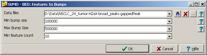
| Data files | Supply a single or a semi-colon separated list of BED files.
Click the "..." button to open a file system browser and select desired files.
More easyly: drag one or multiple files from Windows Explorer into the BED viewer dialog.
Newly dropped files are added to the list of already selected files.
To clear the list, click the "X" button.
To preview the (first) file from the selection list click the "binoculars" button.
|
| Min bumps size | Minimum length for a bump of neighbouring BED objects.
|
| Max bumps size | Maximum length for a single bump of neighbouring BED objects.
If you have huge enriched regions you may get multiple neighbouring / overlapping bumps.
|
| Min feature count | A single bump must have at least this minimum number of features.
|
All selected files are analyzed independantly.
For each input file a new result BED file is created in the same location where the input file was found.
The resultung BED file contains for each bump:
- "#CID" Chromosome
- "Start" Start of bump (BP) within chromosome
- "Stop" End of bump (BP) within chromosome
- "Name" Dummy name (filename)
- "Peaks" Number of original BED objects in the derived bump
(in the example: number of MACS2 γH2AX ChipSeq Peaks)
- "P/MB" number of original peaks per MegaBase
- "Mean coverage" arithmetic mean of "score" from all contained original BED files.
In the example (MACS2 analysis) the "score" column contains the coverage af a MACS2 peak.
- "SDev" Standard deviation of scores from all original peaks.
- "Median" Median of original scores
- "MAD" Median Absolute Deviation (~SDEv for Median)
- "length" of the resulting bump (BP)
An example result file may look like:
track name="Bumps" description="SUMO Bump finder"
#CID	Start	Stop	Name	Peaks	P/MB	Mean-Coverage	SDev	Median	MAD	Length
1	142964908	143464903	NSCLC_1_cell_line-H2aX_broad_peaks.gappedPeak	11	22.0002200022	22.6363639831543	10.7534351348877	18	5	499995	1
1	143164997	143485917	NSCLC_1_cell_line-H2aX_broad_peaks.gappedPeak	12	37.3924965723545	21.5	11.0412454605103	17	4.5	320920	1
4	9218283	9369432	NSCLC_1_cell_line-H2aX_broad_peaks.gappedPeak	12	79.3918583649247	21.9166660308838	7.55234241485596	19	5	151149	4
4	49131786	49571310	NSCLC_1_cell_line-H2aX_broad_peaks.gappedPeak	19	43.2285836495846	22.2105255126953	8.34910774230957	18	5	439524	4
4	49272653	49650909	NSCLC_1_cell_line-H2aX_broad_peaks.gappedPeak	16	42.2993951186498	23.5	8.10760974884033	22.5	6.5	378256	4
5	49406943	49682821	NSCLC_1_cell_line-H2aX_broad_peaks.gappedPeak	15	54.3718600250836	62.2000007629395	73.2863235473633	27	12	275878	5
7	51964259	52432007	NSCLC_1_cell_line-H2aX_broad_peaks.gappedPeak	10	21.3790331546046	16.5	4.71993398666382	15	2.5	467748	7
...
The image shows a zoom-in to a ~8 MB region:
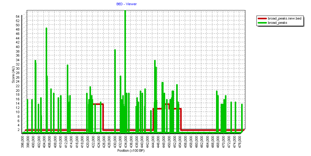
Green indicates the original MACS2 peaks.
Red the resulting "bumps" (applying the above parameters).
BED-tools - 1/2 class test
Lets assume you performed an analysis resulting in a set of chromosmal regions saved in BED format.
Obvious questions would be:
- are there regions conserved between multiple similar samples (replicates) ?
- can i find differences between two (or multiple) groups in different sample groups
The BED-tools class-test allows to perform this analysis using BED files as input.
- Select the BED files for the groups
- Supply files for both groups => 2-class test differential analysis
- Suuply files for group 1 only => 1 class test
- Define the data column used as "intensity" measure (e.g. average coverage from MACS2 bumps).
- Define the resolution.
SUMO divides the genome into small bins with RESOLTUTION number of bases (e.g. 1000 BP).
For each bin (in the eample ~3 Millon 1000 BP bins for the human genome), average / standard deviation
from the groups' members are computed.
- t-test/ANOVA are applied to estimates the individual bin's importance / significance.
t-test are computed with Welsh/Satterthwaite approximation.
- A resultng BED file is created contaiing the union/difference of all regions and their statistical result values.
- Output may be filtered based on the statistical reults.
From SUMO's main menu select Main menu | Utilities | NGS | BED: 1/2 class-test
A parameter dialog opens up:
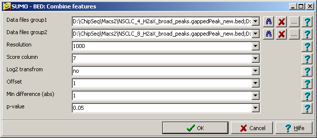
| Data files group1 | Supply a single or a semi-colon separated list of BED files.
|
| Data files group2 | Supply a single or a semi-colon separated list of BED files - ir required.
|
| Resolution | Size of bins in BP.
Resolution downto 100 BP should work.
|
| Score column | The column in all BED files from which the "intensity" information is extracted
and used in the calss test.
To simply count the coverage (coverage of individual samples for a specific bin) define "0"
|
| Log2 transform | Define "yes" to log transform the "intensity values".
But don't forget: for log2 transformation ALL VALUES HAVE TO BE >0
|
| Offset | A contstant to add to the "intensity" values.
Useful to avoid negative number with log2 transformation
|
| Min difference | You may filter bins by
- average "Intensity" (1-class test) or
- differential regulation (2-class test)
Only bins >Min-difference are passed.
Min difference is sign independent.
To bypass this filter supply "0" |
| p-value | You may filter bins by p-value.
Only bins with p≤p-value are passed.
To bypass this filter define p-value = "1"
|
a result file is created:
- with extension "_union" for 1-class tests
- with extension "_difference" for 2-class tests
The result file has BED-4 format and additional columns containing:
- Count,Mean,SDev for the groups
- difference for 2-class test
- t-,p-value, Degrees of freedom
A (unfiltered) result file may look like:
CID	Start	  Stop  	    Name	  Cnt1	Mean1	SDev1	Cnt2	Mean2	Sdev2	C1-C2	M1-M2	t	p	DF
1	2239000  	 2414000  Segment	0	0	0	1	14.12	9.98	-1	-14.12	-1.41	0.126	3
1	2414000  	 2588000  Segment	0	0	0	2	16.94	3.99	-2	-16.94	-6.00	0.004	3
1	2588000 	 2723000  Segment	1	23.71	16.76	2	17.09	3.78	-1	6.62	0.390	3
1	2723000 	 2901000  Segment	0	0	0	2	18.03	2.44	-2	-18.03	-10.42	0.001	3
1	2901000 	 3506000  Segment	0	0	0	1	15	10.60	-1	-15	-1.41	0.12	3
1	10132000	11563000  Segment	0	0	0	1	16.42	11.61	-1	-16.42	-1.41	0.126	3
1	16054000	17324000  Segment	0	0	0	1	16.29	11.52	-1	-16.29	-1.41	0.126	3
1	19411000	19813000  Segment	0	0	0	1	15.30	10.81	-1	-15.30	-1.41	0.126	3
...
BED-tools - Annotate
Certain NGS applications generate results as "genomic ranges", e.g. LAM-PCR applications, ChipSeq peak detection ...
as e.g. SAM or BED files, or variants of those.
Often it will be reqired to annotate individual objects to their genomic context - i.e. annotate these data files.
SUMO expects:
- Annotation file.
Any file with genomic ranges.
E.g. Gene/transcript coordinates, Promoter regions CpG islands,....
- One - or multiple - Data files.
Any file. E.g. SAM, BED, ... All selected files must have same structure.
- All Tab delimited text files
- One object per line
- Genomic coodinates as individual tab separated columns:
- Chromosome (e.g. "chr1", "1")
SUMO will extract the chromosome number ("1".."23","X","Y")<
- Start position on the respective chromosome in BP
- End position on the respective chromosome in BP
- Reading orientation on the cromosome
"+" forward (10000->20000)
"-" reverse (10000<-20000)
- Name of the object
- Order/position of columns can be customized
- Data may be supplied as plain ASCII text or gzip compressed files (coming soon).
SUMO scans each data file against the annotation file and adds annotation informaton to each
feature of the data file (if possibley) in a newly created file.
Depending of the operation mode additonal other files are generated.
Annotation modes
Several annotation models may be used:
Assume we have an annotation file with coordinates for all transcript of a specie.
| Closest | Search the genes with smallest distance to each individual data object.
Independant of orientation of a transcipt, Within. upstream or donwstream of the transcript
Start of end of the feature.
|
| Closest-5' | Only up-stream positon is checked (depending on the transcripts orentation |
| Closest-3' | Only donw-stream positon is checked (depending on the transcripts orentation |
| Regions around Start | Find the transcript where a feature falls into a region around the start of transcript (e.g. promotor region).
Region is defined by Range.
Search region will (be StartTranscript+Range1 .. StartTranscript+Range2.
Define one number (e.g. "2000").
Searh range will be Range1=-2000, Range 2=2000
Or 2 numbers (e.g. "-4000,-2000", thus range1=-4000, range2=-2000).
|
| Regions around Stop | Same as above, but only searching for transcripts at the and. |
| Within | Similar as above.
Search region will cover whole transcript (plus defined ranges, (e.g. Start-4000..Stop-4000) |
For Start/Stop/Within search, additonal data files are generated:
- List of targeted objects (transcripts).
Subset of targeted annotations, additional data columns contain, number and genomic ranges of matching data features.
- Data matrix
indicating distribution of targeted features withing serarch ranges for indivudual annotation object.
You may display the matrix with a heatmap viewer.
Select SUMO | Main menu | Utilities | NGS | Annotate.
A parameter dialog open up:
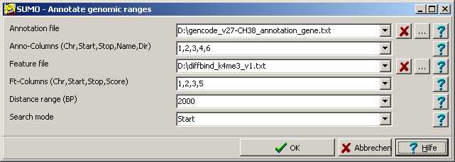
Annotation file
Drag a file from Windows explorer into respective text field, click the "..." button or double click the edit field to open a file selection dialog.
In the demo we created an annotation file containing gene coordinates from data avialabla from Encode project.
The file has a BED6 file format:
##description: evidence-based annotation of the human genome (GRCh38), version 27 (Ensembl 90)	Start	Stop	GeneSymbol	Score	Dir	NN1	NN2	NN2	NN2
chr1	11869	14409	DDX11L1		+	HAVANA	gene	gene_id "ENSG00000223972.5"; gene_type "transcribed_unprocessed_pseudogene"; 	; level 2; havana_gene "OTTHUMG00000000961.2";
chr1	14404	29570	WASH7P		-	HAVANA	gene	gene_id "ENSG00000227232.5"; gene_type "unprocessed_pseudogene"; 	; level 2; havana_gene "OTTHUMG00000000958.1";
chr1	17369	17436	MIR6859		-	ENSEMBL	gene	gene_id "ENSG00000278267.1"; gene_type "miRNA"; 	; level 3;
chr1	29554	31109	MIR1302		+	HAVANA	gene	gene_id "ENSG00000243485.5"; gene_type "lincRNA"; 	; level 2; tag "ncRNA_host"; havana_gene "OTTHUMG00000000959.2";
...
Anno columns
A comma separated list of column-IDs containing the required genomic coordinates:
Chromosome, Start,End,Direction,Name,Score
In the example we would specify "1,2,3,4,6".
Feature file
A single (or muliple) feature files.
Drag files from Windows explorer, or click "..." button or double-click the respective edit field to selecect files.
All simultaneously selected file MUST have same structure.
Data files could be SAM files:
M01688:41:000000000-BGR6Y:1:1101:10374:6013	0	chr11	59327808	22	66S38M136S	*	0	0	GTGTGAC...	FGGGGGGG...	AS:i:69	XN:i:0	XM:i:1	XO:i:0	XG:i:0	NM:i:1	MD:Z:13A24	YT:Z:UU
M01688:41:000000000-BGR6Y:1:1101:12830:7500	0	chr14	77774120	22	63S30M147S	*	0	0	GTGTGAC...	FGGGGGGG...	AS:i:60	XN:i:0	XM:i:0	XO:i:0	XG:i:0	NM:i:0	MD:Z:30	YT:Z:UU
M01688:41:000000000-BGR6Y:1:1101:21160:9931	0	chr19	41748142	22	66S38M136S	*	0	0	GTGTGAC...0	FGGGGGFG...	AS:i:55	XN:i:0	XM:i:3	XO:i:0	XG:i:0	NM:i:3	MD:Z:5A5A22G3	YT:Z:UU
...
(The example shows a few records from a bar-coded LAM-PCR sequencing project. Thus first ~60 bp of the sequences are identical (bar-code, LTR), as well as the quality scores.
For this example we would define the FT-columns as "3,4,4,5".
As the SAM file does not contain explicit end of the feature (implicitely available from CIGAR string), annotion might not be perfect.
(NB: Above SAM filter can create BED formated output)
BED like formats:
Chr	Start	Stop	TotCnt	#Samples	F1	F2	F3  F4...
1	1756351	1756500	31	1	0.000	0.000	0.000	31.001...
1	1781251	1781400	3	1	0.000	0.000	0.000	0.000...
1	4048801	4048950	6	1	0.000	0.000	6.001	0.000...
Here we would correctly define the FT-columns as "1,2,3,4".
Distance range
Define the search range for Start/Stop/Within modes.
Define a single values: Search symmetrically around Eg. Start.
Features falling into the range: Start-Range .. Start+Range will be annotated with this annotation object (e.g. gene).
Define two values: Search in the specified range relativ to e.g. Star.
E.g. try to fnd gene's promoter regions with ChipSeq peaks, you would like to search 2kb regions upstream a gene' (transcript's) start.
Thus you might define distance range "-2000,0".
Search mode
See above.
Result files
For each input file a new file is generated. (Query_FileName_NEW).
Additional data columns are appended to the original file containing matched annnotations.
The eample shows the "annotated" matrix from a LAM_PCR expiment with ~30 samples, "Closest" mode:
Chr	Start	Stop	TotCnt	#Smpl	F1	F2	...	F29	F30    Name  CID  Start  Stop  Dir  Pos  Dist
1	5267701	5267850	281	1	0.000	0.000	...	0.000	0.000	AL139823.1	1  5301928	5301928	-	up	-34078
1	5354701	5354850	79	2	0.000	78.001	...	0.000	0.000	AL139823.1	1  5301928	5301928	-	up	47307
1	5887651	5887800	16	1	16.001	0.000	...	0.000	0.000	NPHP4	5862811	2  5862811	-	up	24840
...
Appended columns contain informaton about "closest" object (in this case gene) from the annotaion file:
- Name - here gene name
- CID - Chromosome number 1..24 (23=x,24=y)
- Start - in BP on respective chromosome
- Stop - in BP on respective chromosome
- Dir - "+" = forward orientation of gene on chromosome, "-" reverse orientation
- Up - feature is found around/upstream start of gene
Down - feature is found around/downstream end of gene
- Dist - distance in BP relative to
- Start (upstrema) or
- stop (dwonstream) of the closest gene.
Objects file
For each input query file a new feature file is generated (QueryFileName_objects):
| CID | Start | Stop | Name | Dir | Cnt | Locs |
| 1 | 175123 | 1780457 | NADK | + | 2 | 1756351,1756500;1781251,1781400; |
| 1 | 4012921 | 4019508 | AL805961.2 | - | 1 | 4048801,4048950; |
| 1 | 5301928 | 5307394 | AL139823.1 | + | 2 | 5267701,5267850;5354701,5354850; |
| 1 | 5862811 | 5992473 | NPHP4 | + | 1 | 5887651,5887800;6037351,6037500; |
| 1 | 6834333 | 6834618 | AL590128.1 | - | 1 | 6834601,6834750; |
| ... |
The file contains a list of annotation "objects" (genes) wich were hit by the features from your data files.
One object per line.
For each object tab-delimited
- CID - Id of chromosome (1..24)
- Start - in BP
- Stop - in BP
- Name
- Dir
- Cnt - Number of features mapped to this object (gene)
- Locs - list of genomic coordiantes of mapped features
Coverage matrix
For each input query file the coverage by the mapped features of targeted objects (genes) is generated (QueryFileName_covmat):
The matrix - a tab-delimited text - file accumulates for each targeted annotation object (gene),
the distribution of mapped features accross the search range.
Obviously, it only makes sense to generate such a matrix for objects with same size (i.e. Start/Stop search modes.
The matrix may be displayed like a gene expression heatmap:
A set of tools to work with SAM/BAM files
Generate some diagnostic data / plots from SAM/BAM file.
Selet SUMO main menu | Utilities | NGS | SAM-tools | SAM/BAM-QC.
A parameter dialog opens up:
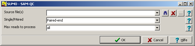
| Source files |
Supply a list of files (separated by semicolon ";") to be processed.
Click the "..."-button to open a file system browser.
Select one or multiple files.
Alternatively drag one or multiple files from Windows explorer into Source files text field.
Presently you may use the file types:
- SAM files (file extension ".sam") or gzipped sam files (".sam.gz")
- BAM file ".bam"
- FastQ (".fastq") or gzipped FastQ (".fastrq.gz")
Click the binocular button to preview SAM/FastQ files (not for BAM files).
I.e. just view the first view thousand lines from the file.
|
Single/Paired
|
| Max reads to process |
Often it is enough to analyses a part of the reads (e.g. a few million reads).
This may already give indication for:
- base compostion biases - not properly removed adapter sequneces
- overrepresentation of chromosomes, MT, not assigned contigs - cloning / ampification artifacts
- correctly mapped reads - genomc rearrangements, chimeric reads, low qulity mapping
- ...
Specify the number of reads to process from each file (e.g. "1000000").
Select "all" or leave the field empty to process the whole file.
|
For each of the selected files a report file (extension Aold_Fileanme_SSAM-QC.htm") is generated in the
same folder where the source file is located.
See a demo file.
The analysis sections
:
Basic statistics about you data file, e.g.:
Filename="D:\Demo_R1.fastq.gz_Aligned.out.sam.bam"
Total number of sequences: 7.600566 [MegaSeq]
Total number of bases: 0.943 [GigaBP]
Number of UNIQUE mapped sequences [Mega]:	3.304229	(43.47%)
Number of UNIQUE qualified mapped sequences [Mega]:	3.304229	( 43.47%)
Number of bases [Giga]:	0.410	( 43.47%)
AT-Content (%): 47.96
CG-Content (%): 52.03
Depending on data preparation (e.g. adapter trimming) and mapping (softclipping of not aligning sequence parts)
length of individual sequences may vary.
A strong variation of sequences from the expected length after the sequencing run may indicate problems during
cloning / amplification / sequencing / mapping.
The graph shows the normalized density distribution as well as the cumulative distribution:
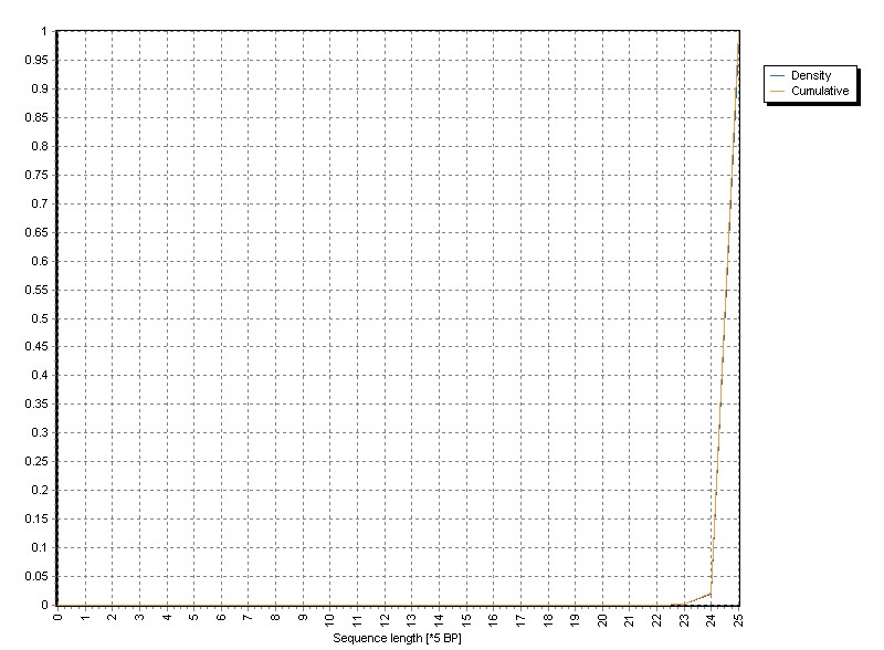
The example was sequenced with 125 bp.
The length variation mainly originates from soft clipping by BOWTIE2 mapper.
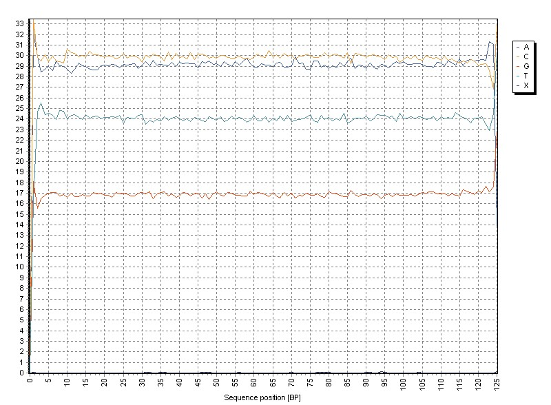
Here we analyze the base composition per sequence position across all reads in the SAM/BAM file.
The "X"-series contains all ambiguity characters (e.g. "N", ...).
A priori, one would expect a more or less constant distribution of bases across all sequence positions.
(At least with whole genome / transcriptome sequncing).
Local inhomogenities may indicate contaminations with not properly removed adapters / bar-code sequences ....
The sample shows:
- A strong base specific bias in the range BP 1-13 and BP 113-125
- Overrepresentation of C in the range BP 14-30
- Overrepresentation of G in the range BP 75-112
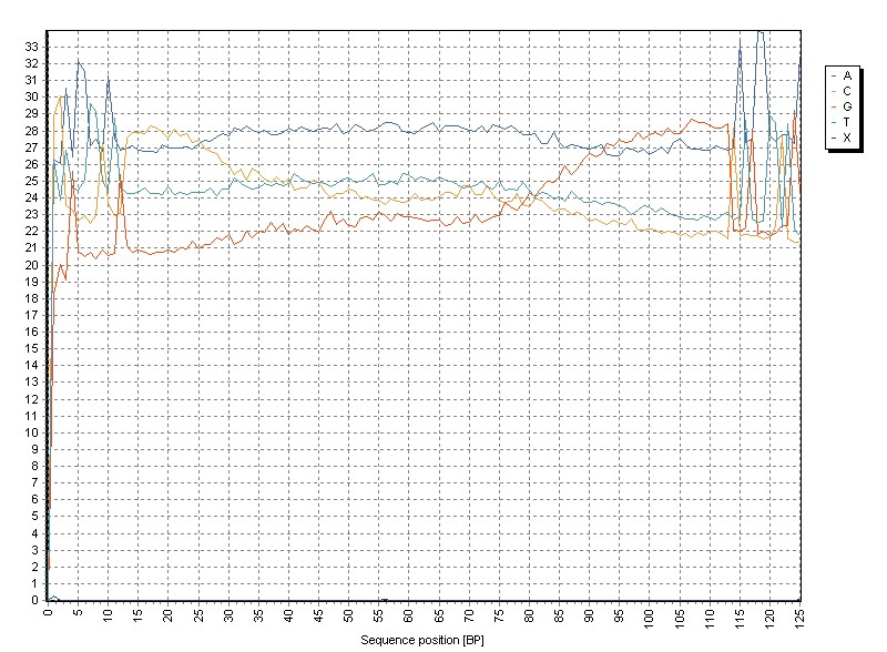
Removal of adapter sequences removes these biases:
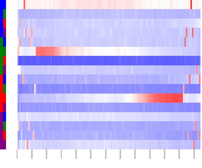
Additionally, colormaps visualize distribution of Di-/Tri-/Tetra-nulceotides across the sequence positions:
Di-Nucleotides:
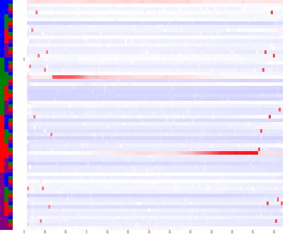
Tri-Nucleotides:
Tetra-Nucleotides:
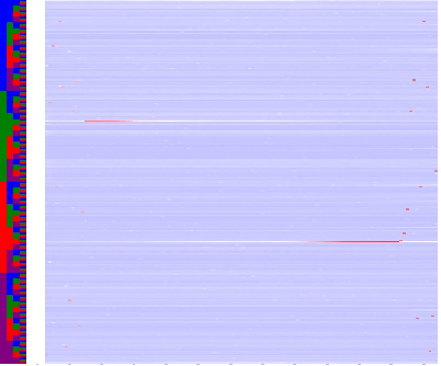
The colored Columns at left side of the map encode the base sequence: ACGT.
The map colors indicate: ------- =over-represented,
------- =under-represented,
The gray ticks below at the bottom of the maps indicate base position, starting with one, 10 BP increments.
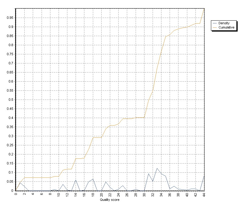
Most sequence mapper tools (e.g. BOWTIE, BWA) generate mapping quality values, indicating the significance of a mapped sequence.
A priori, one would hope that the vast majority of the newly generated sequences map correctly (e.g. MapQ>30) to the reference.
Only a smaller fraction of sequences should contain many discrepancies to the reference or should onyl partially match to the reference (e.g. chimeric sequences).
Structural variants like SNPs should not drop the MapQ values dramatically, chromosomal aberrations or rearrangements should only affect a very small fraction of the new reads.
The graph show density as well as cumulative distribution of Mapping Quality values:
In paired end reads, SAM/BAM files contain information about length of the region spanned by correctly mapped mate (read) pairs.
The extracted target length distribution should match the sequencing library size distribution.
The graph shows normalized density- as well as cumulative distribution of target lengths from all read pairs:
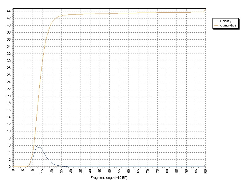
All target sequneces larger 1000 BP are aggregated in te the 1000 BP channel of the histogram.
For single-end sequencing this analysis is meaningless - and therefore not shown.
The number of soft clipped bases is read from the CIGAR string contained in the SAM / BAM files.
A priori one would expect thit clipping of seqences should hardly occur in case all adapter sequneces have been completely removed from the sequences before mapping.
The distribution of left, soft-clipped bases is shown in the graph, both as density as well as cumulative distribution:
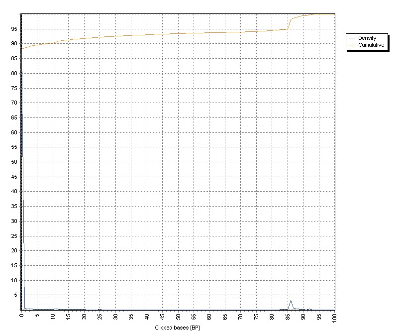
The demo graph shows soft clipping from a not correctly prepared sample.
More then 10% of the sequences contain clipped sequences up to 80 PB in length. These conatmination origin from not correctly removed adapter sequences.
Similar to above, the distriubtion of sequneces clipped from the right end of th sequences is shown.
Again, a mentionable proportion of long clipped sequence regiosn may indicate not properly prepared sequences (adapters, ...).
Like above, the graph visualizes both, density as well as cumulative distribution of right soft-clipped bases.
The graph shows the distribution of reads mapped to chromosomes.
Channels "0" contains all sequences not mapped to any chromosme.
"1" to "22" represent the autosomes.
"23","24" the X and Y chromosome.
"25" the Mitochondrial genome.
Alternative mappings are assigned to the "0" channel.
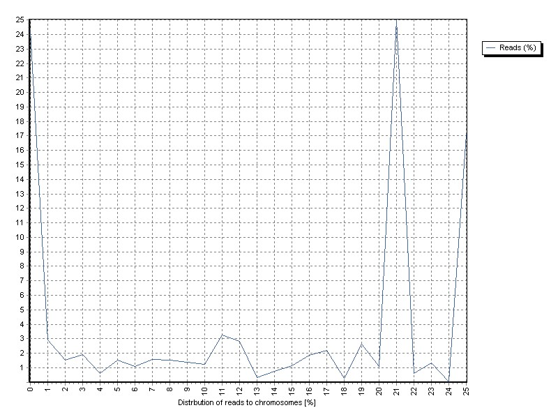
A priori one would expect a rough correlation between chromosome size and fraction of mapped sequences (especially with genome- and exome-sequneces).
The sample shows a high overrepresentation of chromosome 21 (~25% of allreads).
A more detailed view uncovers the overrepresented region Chr21:8,200,000-8,400,000.
This region contains ribosomal s28 gene, indicating that ribosomal RNA depletion during sample preparation failed.
In case the reads where nt mapped against a (human) reference genome, this grpah is meanngless.
Data processing may take a while:
- ~150000 reads/s from fastq /SAM files
- ~ 70000 reads/s from GZ-compressed / BAM files
(On an I7-3930, 3.2GHz, 1 thread, data on local spinning disk.)
Typical file size is < 2 MByte.
Each report file is a single html document containg all graphs as in-line jpg-images.