tSNE
tSNE computes internally a two dimensional probabilty distribution map of pairwise vector similarities.
A output 2D map - the tSNE-graph - is generated.
In an iterative process, the data points on the output map are moved to minimize the Kullback-Leibler divergence between these two maps.
t-SNE may be better suited to model the small pairwise distances betweeen data vactors and thus may be better to visually explore the result data and find structure / clusters of similar objects.
On the other hand, the neighbour embedding does not necessarily reflect real magnitude of similarity between individual data points / clusters.
Therefore, tSNE-maps should be compared with other "embedding" techniques (e.g. PCA, clsutering).
For more details about tSNE see L.J.P. van der Maaten and G.E. Hinton. Visualizing High-Dimensional Data Using t-SNE. Journal of Machine Learning Research 9(Nov):2579-2605, 2008.
or a basic introduction into t-SNE; Paper Dissected: "Visualizing Data using t-SNE" Explained.
SUMO does not use an own implementation of tSNE but utilizes the improved FFT-accelerated Interpolation-based t-SNE (FIt-SNE) version implemented by Linderman et al. (2017).
To ensure compatibility, SUMO uses "FItSNE-Windows-1.0.0", from Dec-2018, downloaded from their web-site and mirrored on SUMO web site.
t-SNE with SUMO
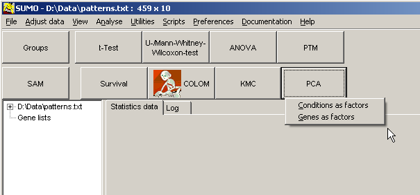
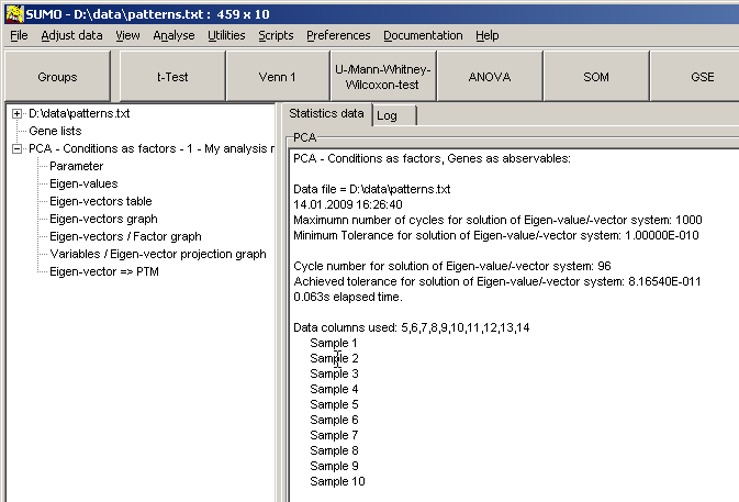
Load a data matrix.Click the PCA / t-SNE-button or select Main menu | Analyses | PCA / t-SNE.
Select to run a t-SNE analysis with either Genes (row-vectors) or Conditions (column vectors).
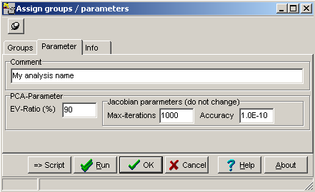
A parameter dialog opens up, allowing to set of few FItSNE processing parameters:
| Max number of iteration cylces |
Number of cycles, FItSNE tries to optimize positioning the output vectors. A larger number of iteration may generate a more accurate map, in case FItSNE finds a local optimal solution. Most simply, run FItSNE with a decent number of iterations (e.g. 250). In case the mapping looks non informative, try to run it again with more iterations (e.g. 500 next round 100, ...). Better, run FItSNE on the command line and see its progress dependong on the iterations. |
| Perplexity: | A larger perplexity will tend to spread the data clouds. Try different values and observe the outcome. But: recommended Perplexity = (Number_of_Features_Conditions - 1) / 3). I..e. 30 samples => Perplexity ~10. SUMO automatically adjusts a too high perplexity accordingly. |
| Dimensions:' | Generate a 2 dimensional embedding => data clouds in a 2d-plain (commonly used model) or a 1-dimensional embedding => stacked bars |
SUMO generates a FIt-SNE specific data file, saves it in the folder where SUMO executable reside, und starts FItSNE.
FItSNE requires numeric data - obvious.
Thus, you should impute non-numeric values in your data matrix prior to running FItSNE.
In case /SUMO finds non numeric values while writing the FItSNE data file, it will finally replace NANs by ZERO.
In case of very few randomly distributed NAN cells, this will most probably not interfere with the mapping.
Larger number of NANs concentrated in singular data rows/columns or even correlating with data structures may introduce biases and thus artificial mappings.
Depending on data size (i.e. number of data vectors, length of data vectors) and internal data structure, FItSNE may require a while to process the data.
Some timings with random data, I7-3930, 3GHZ, 12 hyperthreads, 32 GB RAM:
| Number of vectors | Legth of vectors | Consumed RAM (GB) | Elapsed time (s) |
|---|---|---|---|
| 100000 | 1000 | 2.8 | 270 |
| 10000 | 1000 | 0.3 | 30 |
| 1000 | 1000 | 0.03 | 15 |
| 1000 | 10000 | 0.3 | 45 |
| 1000 | 100000 | 2.5 | 65 |
Thus, be patient and wait until FIt-SNE has finalized.
Although in principle possible, it may be wise not to run other SUMO functionality while waiting for FIt-SNE.
You may terminate FIt-SNE by clicking the Break button or press ESC-key.
As soon as FIt-SNE has finalized, SUMO will pick up FIt-SNE binary result file.
It converts and stores result data into a tab-delimited text file ("SUMO-path\fitsne.txt) which may be used anywhere.
The tab-delimited text file contains the mapping coordinates in the first two data columns, as well as feature/sample annotation in the third columns (multiple annotation separated by ";".
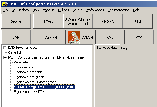
Furthermore, SUMO shows FIt-SNE mapping in it's Scatterplot viewer:
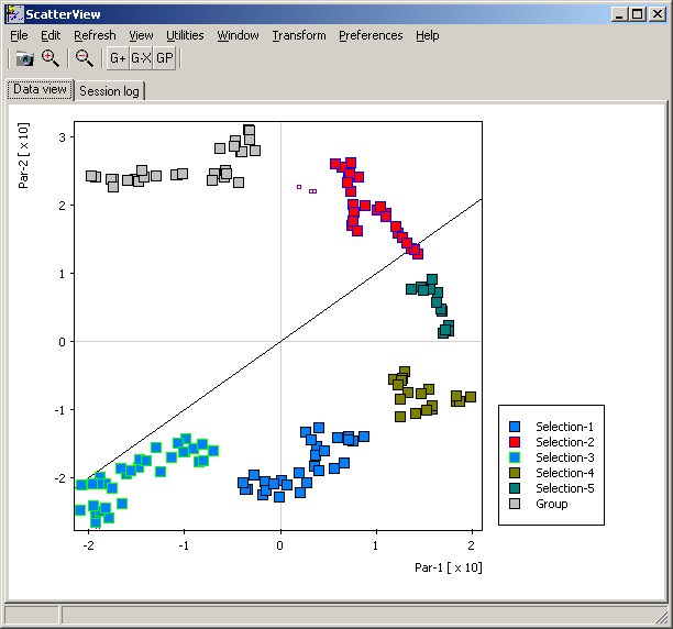
All annotatins are passed to the Scatterplot viewer too.
Thus you may search for certain data (Scatterplot main menu | Find) or draw selection ROIs and review contained data points and their annotations:
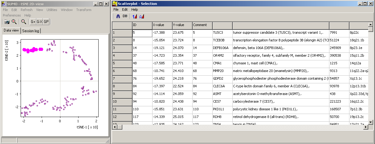
You may also load addtional values for the data points (e.g. regulation, intensity, ...) and show them as indivdual data point's color, size (Scatterplot main menu | Paste data | Size/Color.
But take care that pasted data have exactly same order and size as map data.
See more details about Scatterplot viewer.
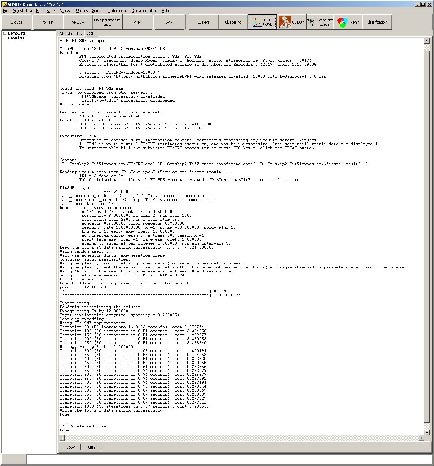
Finally the process-report as well as an error-report (if errors occurred) from FItSNE is shown in the message/Log tabshet:
In case the tSNE mapping is not informative, this processing output may contain hints how to adjust FIt-SNE parameters.
UMAP
In a first step, UMAP computes similariteis between all data vectors (using distance metrics well known from hierarchical clustering) and filters most relevant interactons.In a second step these interactiosn are embedded in 1-/2-/3-D space applying a "force-feed" method similar to network building (e.g. gene-networks).
For more details about UMAP see:
Leland McInnes, John Healy, James Melville.
UMAP: Uniform Manifold Approximation and Projection for Dimension Reduction
arXiv:1802.03426 [stat.ML]
or a basic introduction into UMAP including several samples on GitHub.
SUMO does not use an own implementation of UMAP but wraps the Python based implementation from Leland McInnes, John Healy, James Melville.
This requires installation of Python, the UMAP package as well as any additional underying Python packages imported by UMAP.
We recommend to install Python / UMAP via ANACONDA / Miniconda.
Installation of ANACONDA
Goto to
During installation you may select between installation only for the current or for all users:
- Current user - no administrator account required for installation.
Install outside a Windows user account's folders (NOT: Deskttop, Own documents, ...) but on a public avialable folder (e.g. second data drive).
Thus the installation of ANACONDA may be used by any user on this computer.
Other user must create links to ANCONDA on their own. - All users - Install by adminsitrator. All users of this computer may access ths ANACONDA installation.
Install UMAP
After successful installation of ANACONDA open an ANACONDA prompt fron Windows's start menu.
Install UMAP by typing:
conda install -c conda-forge umap-learnor
conda install -c conda-forge/label/cf201901 umap-learnANCONADA now will download UMAP as well as all other required Python packages.
Setup ANACOND Proxy server:
In case your computer system accesses the Internet via an institutional proxy server, installation may fail.
Then it may be necessary to tell ANACONDA about this proxy prior to installation of new packages.
See here how to configure ANACONDA.
In brief:
- Use a text editor (eg. Windows' notepad.exe) to create a configuration file in your users home directory:
E.g. "c:\users\myAccount\.condarc"
Replace "myAccount" with the respective user account name.
".condarc" MUST be used, don't forget the leading "."
- add the proxy definition:
proxy_servers:
  http: http://user:pass@corp.com:8080
  https: https://user:pass@corp.com:8080
Replace "corp.com" with the name of your organisation's proxy server
Replace "8080" with your organisation's proxy port number
If your organisation's proxy requires authentication replace "user:pass" with your username:password
If your organisation doesn't require proxy authentication - skip user:pass
- Save the file.
Now ANACONDA should be able to access its repositories for software installation.
UMAP with SUMO
Load a data matrix.Click the PCA / t-SNE / UMAP-button or select Main menu | Analyses | PCA / t-SNE / UMAP.
Select to run a UMAP analysis with either Genes (row-vectors) or Conditions (column vectors).
A parameter dialog opens up, allowing to set UMAP processing parameters:
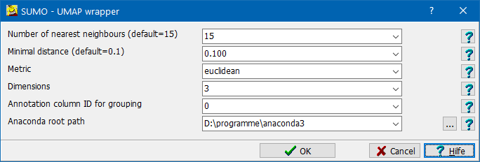
| Number of nearest neighbors |
|
| Minimal distance | |
| Dimensions: | Define number of dimensions for embedding: 1 - dimensioanl embedding 2 - dimensional embedding => data clouds in a 2D-plain (commonly used model) 3 - dimensional embedding => data clouds in a 3D-space |
| Metric | Method how to compute similarity / distance between data vectors. Choice of a metric may fudamentally alter resulting embedding. Thus consider carefully which metric to use depending on the data, the experimental design and the scientific question. |
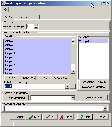
| Annotation column ID for grouping |
Data viewers will use this annotation column to auto group (genes/conditions). The annotation column should contain a small set (~≤<100) of "class identifiers" (e.g. treatment names). Specify "0" or leave empty to avoid autogrouping. |
| Anaconda path | Specify location of your ANACONDA, or any other Python installation Click the ... button to open a file system browser and navigate to the repective folder. |
Click the OK button to lauch UMAP.
SUMO performs the steps:
- Write processing parameters and data into a Comma Separated Values file (.csv).
A file ("SUMO_umap_data.csv") is created in the folder were SUMO.exe is located.
- Generate a Python script to perform UMAP analysis.
A file ("SUMO_umap.ps") is created in the folder were SUMO.exe is located.
- Create a Windows command script to set the ANACONDA environment and launch the analysis.
A file ("SUMO_umap.bat") is created in the folder were SUMO.exe is located.
- Wait until UMAP has finalised.
Although in principle possible, it may be wise not to run other SUMO functionality while waiting for UMAP to finalize.
You may terminate UMAP at any time by pressing ESC-key or clicking the Break button.
- Load and display results as 2D-/3D-scatterplots
Data are read from TAB-delimited result ("SUMO_umap_resut.txt") file created by the "SUMO_umap.ps" Python script.
- Info / Error-Messages from the scripts / UMAP / Python are show in SUMO's Log tab-sheet.
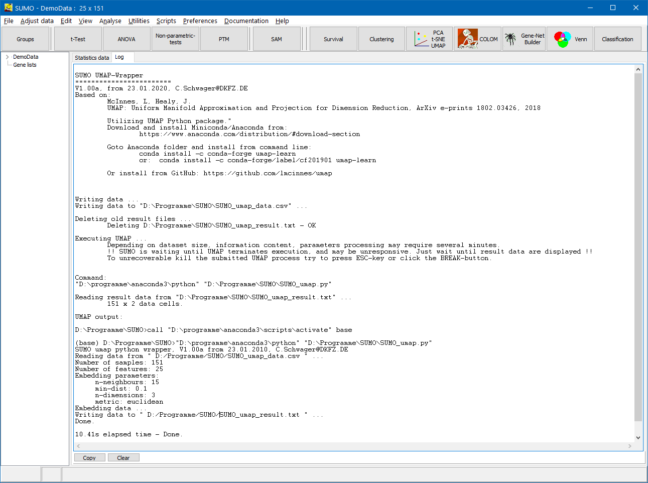
SUMO generates a UMAP specific data file, saves it in the folder where SUMO executable reside, und starts UMAP.
UMAP requires numeric data - obvious.
Thus, you should impute non-numeric values in your data matrix prior to running UMAP.
In case /SUMO finds non numeric values while writing the UMAP data file, it will finally replace NANs by ZERO.
In case of very few randomly distributed NAN cells, this will most probably have low iimpact on the embedding.
Larger number of NANs concentrated in singular data rows/columns or even correlating with data structures may introduce biases and thus artificial mappings.
Depending on data size (i.e. number of data vectors, length of data vectors) and internal data structure, UMAP may require a while to process the data.
Some timings with random data, I7-8700k, 3.4 GHZ, 12 hyperthreads, 64 GB RAM:
| Number of vectors | Legth of vectors | Elapsed time (s) |
|---|---|---|
| 100 | 100 | 5.27 |
| 1000 | 100 | 7.63 |
| 10000 | 100 | 31.67 |
| 100000 | 100 | 171.53 |
| 100 | 1000 | 6.11 |
| 100 | 10000 | 11.83 |
| 100 | 100000 | 68.28 |
Thus, be patient and wait until UMAP has finalized.
Like with any othe similarity based data partitioning method, unspecific background signals or very low intensity noisy data may - in the best case - not be helpful for embedding but only consume CPU time.
In the worse case they can introduce biasis which may even generate meaningless sub-structures in the final embedding.
Some samples:
Graphs are generated from SUMO's internal "Intensity" demo data set, applying UMAP to genes:
1-D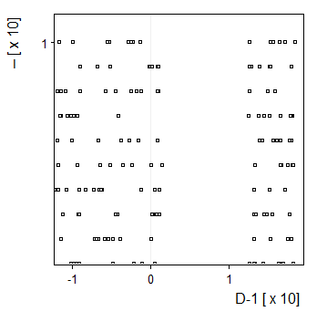 Here, Y-Dimension is meaningless. |
2-D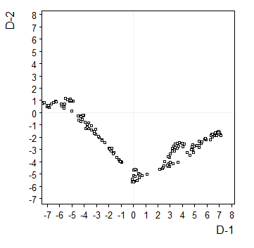 |
3-D |
Embeddings in different dimensions may suggest different sub-structures.
Embedding parameters may influence the embedding, e.g. metric:
| Euclidean |
Canberra |
Cosine |
Correlation |