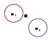
| Class | Count |
|---|---|
| T1 | 2 |
| T2 | 3 |
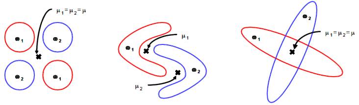
Thus we would assign the new sample to class 2 with KNN classification.
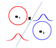
In opposite to Closest Centroid/LDA: there, we would assign the sample to class 1.
Obviously, KNN may be better suited to predict non-homogenious non symetric training data sets.
ANN - Artificial Neural Network
SVM - Support Vector Machines
RF - Random Forests
The original publication summarizes:"Random forests are a combination of tree predictors such that each tree depends on the values of a random vector sampled independently and with the same distribution for all trees in the forest. The generalization error for forests converges a.s. to a limit as the number of trees in the forest becomes large.
The generalization error of a forest of tree classifiers depends on the strength of the individual trees in the forest and the correlation between them. Using a random selection of features to split each node yields error rates that compare favorably to Adaboost (Freund and Schapire[1996]), but are more robust with respect to noise. Internal estimates monitor error, strength, and correlation and these are used to show the response to increasing the number of features used in the splitting. Internal estimates are also used to measure variable importance. These ideas are also applicable to regression."
From the original publication:
LEO BREIMAN
Random Forests
Machine Learning, 45, 5-32, 2001, Kluwer Academic Publishers.
SUMO utilizies Ranger64 Version 0.2.7, a standalone C++ implementation of random forests:
On safari to Random Jungle: a fast implementation of Random Forests for high-dimensional data
Daniel F. Schwarz, Inke R. König and Andreas Ziegler
Bioinformatics, Volume 26, Issue 14, Pp. 1752-1758.
The basic part of a random forest is a decision tree.
Lets look at a simple example.
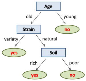
A decision tree with low complexity to predict whether an Apple tree will bear fruit.
|
As input, the tree requires a vector containing information about the attributes of an Apple tree (e.g. age of the tree, strain: natural or variety, rich or poor soil). Starting with the root node of the decision-making rules of the tree be applied to the input vector. At each node one of the attributes of the input vector is queried. In the example, at the root node the age of the Apple tree. The answer decides: old=>no fruit, young=>proceed to next node. After a series of evaluated rules, you have the answer to the original question. Not always, all levels (nodes) of the decision tree must be traversed. |
 |
How to build a decision tree (automatically) from a suited date set?
E.g. the set of genes best suited to distinguish two phenotpes ?
One method could be a recursive top-down approach.
It's crucail to have a suitable record of reliable empirical data to the decision problem (the training data set). The classification of the target attribute must be known to any object (sample) of the training data set.
In each iteration step, the attribute which best classifies the training samples will be identified and used as the a node in the tree.
This is repeated until all samples from the trainng set are classified.
At the end, a decision tree is built, who describes the experience and knowledge of the training data set in formal rules.
One problem could be, that thew decision tree becomes overfitted - it can exactly and perfectly classify the training set- but fails with other data.
To circumvent this problem a randomisation with subsampling is applied:
A variety of random subsample of attributes as well as of traing samples is used to build multiple decision trees.
Mutliple random decision trees are grown and combined to the random forest.
From this random forest, we can deduce weight factors for the individual attributes and extract an "averaged" decision tree which should be able to classify our class of problems.
(Adopted from Wikidpedia))
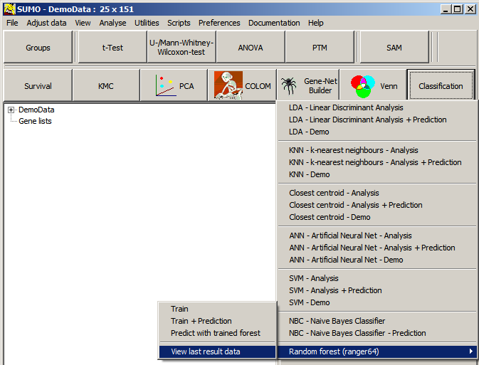
Select the respective Random Forest method from SUMO's classification menu.
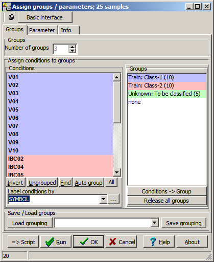
Define the sample groups according to the seleted method:
- Training: 2 or mopre groups groups (Class1, Class2, ...)
- Training + Predicition (Class1, Class2, ... + Query)
- Prediction with forest : 1 group (Query)
NB: - Query data set should contain the same features in same order as the training set
- Use the same parameters as used in the training
A parameter dialog opens up:
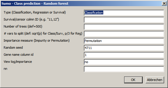
Set the parameters accordingly:
| Type | Prediction method:
|
| RegressionSurvial/censor column ID: - Regressiona: the annotation row ID containing the numerical parameter for regression analysis - Survial: specify spevify comma seaprated: + surval row ID - time to evnet (typical time to death of sample) + censor row ID - defines whether sample experienced event > NOT censored ( value = 0,no,not,false) sample did NOT experience event => sanmple censored (value=1,yes,ja,true) | |
| Number of trees | Number of random trees to grow
|
| # vars to split | At each branch of the decision tree, only a part of the variates (features) is used for classification. |
| Importance measure | Method how to measure influence of the individual features on the overall classifier |
| Random seed | Multiple Random decision trees are grown random selected trraining data subsets and combined.|
| Gene name column ID | ID of gene annotation column containing unique Gene / Feature names / IDs These IDs show up in the importance file. |
| View log/importance | Yes/no : Automatically show Ranger64 log and importance file. |
| Forest file name | Define name and path to forest file generated / used in ther present run Default: "ranger.forest" |
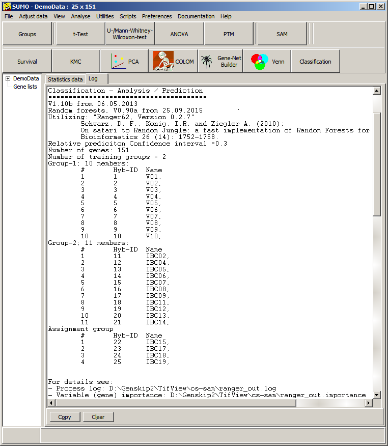
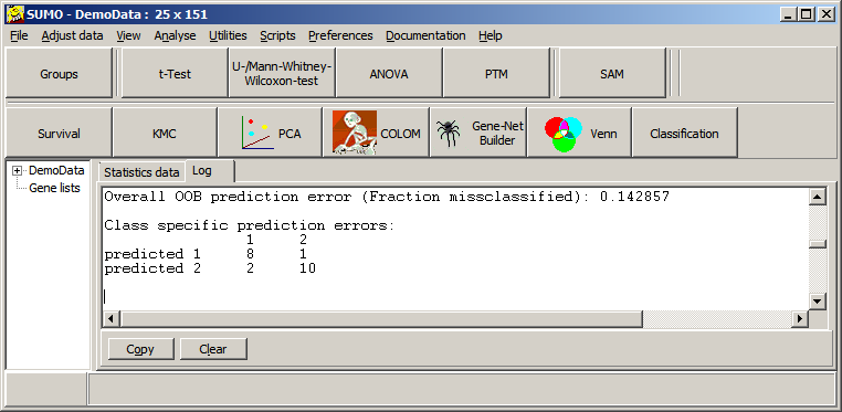
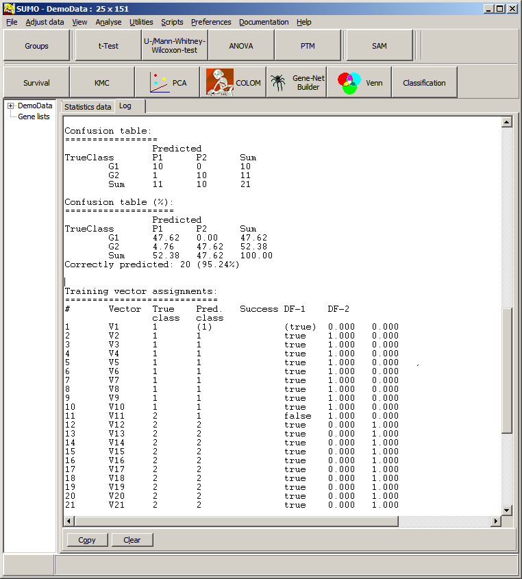
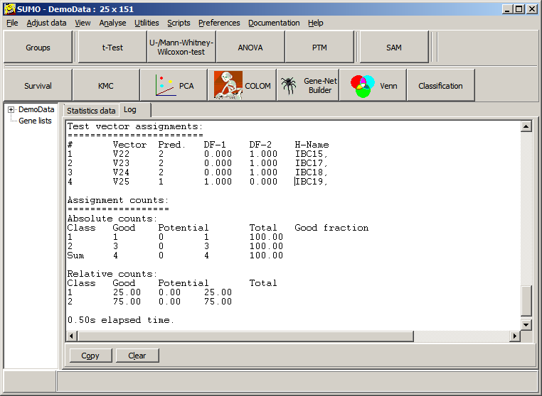
Now, Ranger64 is called to build the forest and SUMO harvests the results to the Log-tabsheet - see above.
Several data files are created in the folder where SUMO.exa as well as Ranger64.exe are localized.
The forest
A binary representation of the extracted decision tree.
The forest file may be reused to classify new samples without the time consuming recomputing of the forest again.
New samples for predicition should have:
- same number and order of features
- same platform (e.g. transcriptome array)
- same data normalization / transformation.
It might be not recommended to apply a RF deduced from virtual-pool-normalized/log2-transformed gene expression array ratios to rlog transformed RNASeq counts.
The importance file:
A tab-delimited list of importance values for each feature in the training set.
Each line contains the features name (=> Gene name column ID) and its respective importance values.
High importance values indicate high correlation of the particular feature to the grouping/regresson: they are helpful for classification.
Features with importance value ~0 are not helpful for classification
Features with importance value << 0 are contraproductive
Thus it may be helpful to filter the importance file, as well as traing data set und later test data sets for high impotant features.
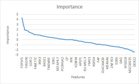
The graph shows the sorted importance values from a small gene expression data set (nb. not all gene names are shown on the x-axes).
- the break point at importance ~2
- or the plateau at importance ~1
may indicate positions, where to filter the most valuable features for later classification.
Now you may generate a new RF from the filtered training set and use to predict new filtered test data sets.
Furthermore, the highly important features may be regarded as most singnifcant features of a kind of non-parametric test (class-test/regresson response).
Trouble shooting
In case classification didn't succed or results seems to be weired, view all Ranger64 data files.Select View last result data from SUMO's classification menu.
All result files are opened with Windows' Notepad.