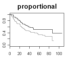
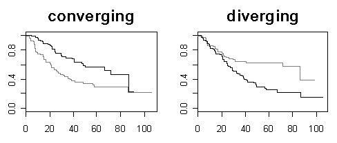
| Gene selection in microarray survival studies under possibly non-proportional hazards Daniela Dunkler, Michael Schemper and Georg Heinze Bioinformatics, Volume 26, Issue 6, Pp. 784-790. |
install.packages('survival')
install.packages('coxphw')
R may ask you to select an R-mirror site. Select the geographically most closest one.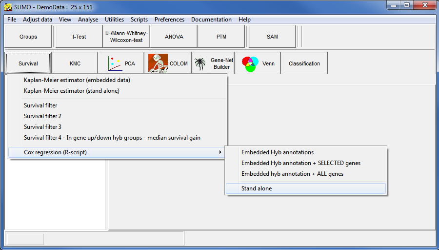
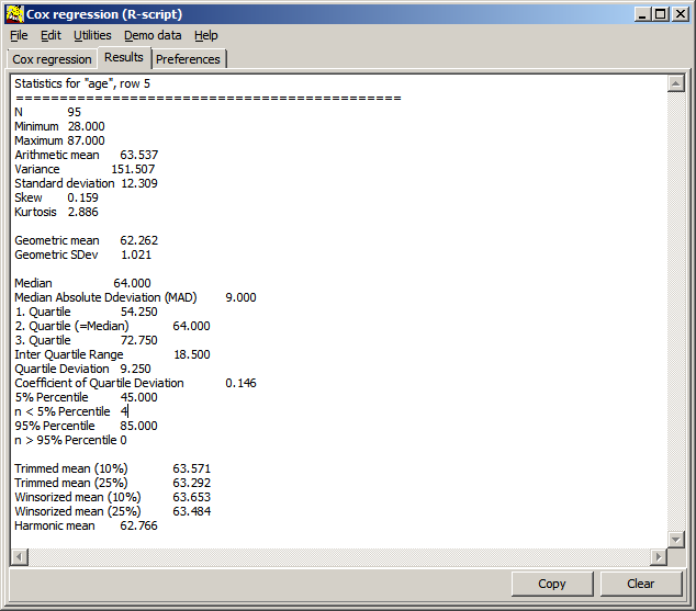
| n | Number of values analysed |
| Minimm | Smallest value in dataset |
| Maximum | Largest values |
| Arithmetic mean | |
| Variance | |
| Standard deviation | |
| Skewness | Assymetry of the data set (3. distribution moment) |
| Kurtosis | Peakedness of the dat set (4. distribution moment) |
| Geometric mean | Meaningful for ratio data |
| Geometric SDev | |
| Median | Robust, outlier insensitive average |
| Median Absolute Deviation | |
| 1. Quartile | Value at lowest 25% of the data set |
| 2. Quartile | = Median |
| 3. Quartile | Value at highest 25% of the data set N.b: Boxplot often illustrate the 1.-3.-Quatile data range |
| 5% Percentile | Value at lowest 5% of the data set |
| n < 5% Percentile | Number of data values smaller 5%-Percentile |
| 95% Percentile | Value at highest 5% of the data set N.b.: The Whisker in a Box-Whisker plot often illustrates the 5%-95%-data range |
| n > 95% Percentile | Number of data values Larger 95%-Percentile N.b.: In a Box-Whisker plot often <5% as well as >95% are often displayed as min/max data points. |
| Trimmed mean (10%) | Robust, outlier insensitive average |
| Trimmed mean (25%) | Robust, less outlier insensitive average |
| Winsorized mean (10%) | Robust, outlier insensitive average |
| Winsorized mean (25%) | Robust, less outlier insensitive average |
| Harmonic mean |
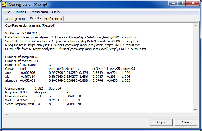
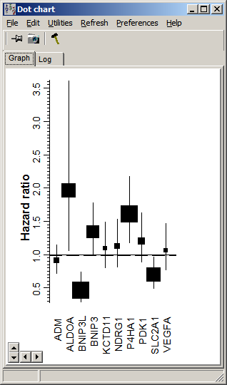
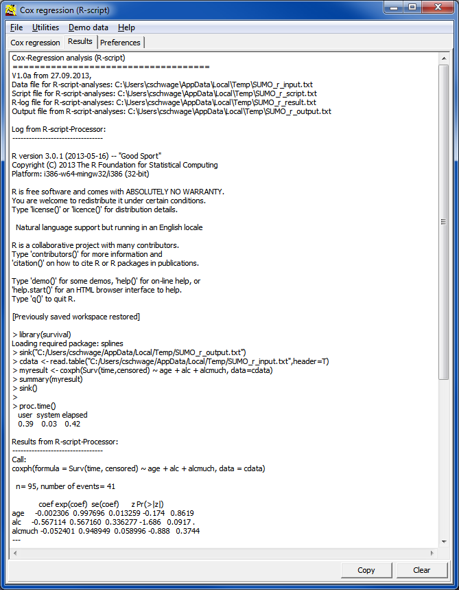
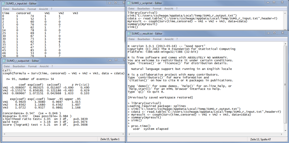
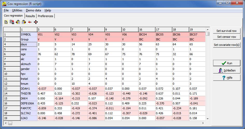
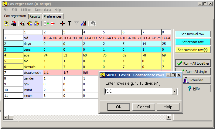
| Covar | Name of covariate, as defined in the input data table / file | |
| coef | regression coefficient of the log model | |
| exp(coef) | regresson coefficient => Hazard ratio which tells us wether the probability to experience the "event" is increased (>1) or decreased (<1). | |
| se | Standard error of hazard ratio | |
| z | z-score | |
| pr(>|z|) | probability value which tells us, whether the finding is statistically significant (e.g. p<=0.05). | |
| Lower/Upper.95 | 5% confidence interval for hazard ratio |