The Kaplan-Meier
estimator estimates the survival function from life-time data.
But the formalism may be applied to analyze / visualize the probability of any
event to occur after a certain time point (e.g. death of patient after certain
treatment, failure of hard disk in computers, ...). Or even something completely
different (e.g. probability of a tree to break depending on height, ...).
For more details about Kaplan-Meier estimator visit
Original publication:
Kaplan, E.L. & Meier, P. (1958).
"Nonparametric estimation from incomplete observations".
Journal of the American Statistical Association 53: 457–481.
To estimate the probability that two data sets show the same time dependency, the Logrank test can be performed.
Assume you have in your condition annotations both
survival data, i.e. time interval (number of weeks, month) which the patient survived or until the patient is lost from the study
censoring data, i.e. a flag whether the patient died or was lost from study
in two separate data rows within the header, then you can easily generate Kaplan-Meier diagrams.
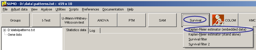
Click the Survival button and select Kaplan-Meier estimator (embedded data):
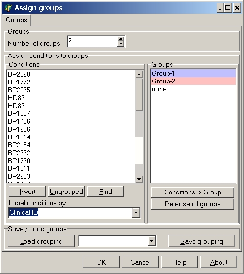
Select the desired number of groups and assign hybridisation to the respective groups (for more details how to build groups go here).
NB!! Hybridisations can UNIQUELY be assigned to one group only NB !!
Select the parameters tab:
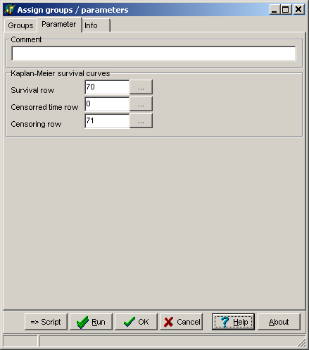
Specify:
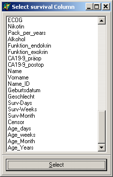
| Survival row |
The line number in your data matrix where survival data
(or data when a patient was lost from the study) are found. |
| Censoring row | A line which contains flags telling SUMO whether the patient
|
Click the OK button.
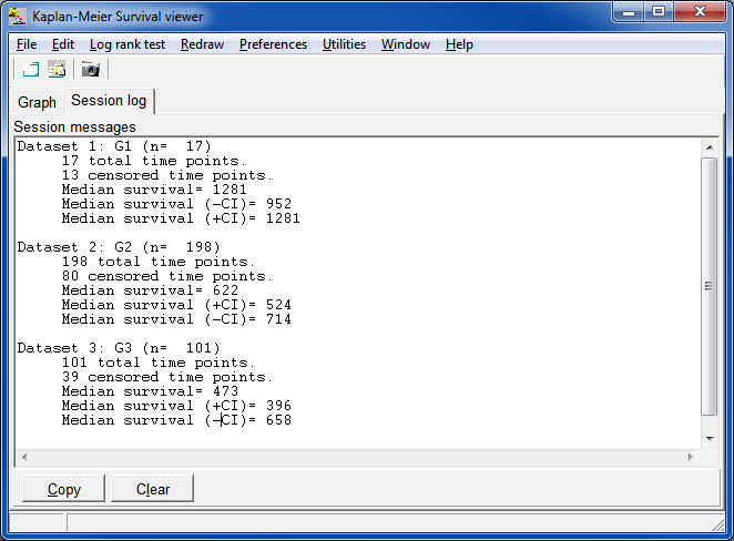
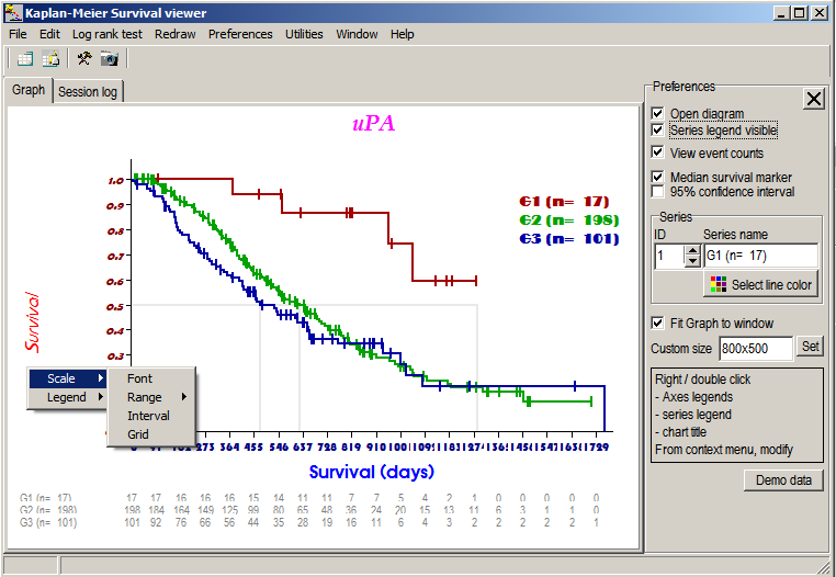
Now the Kaplan-Meier survival graph for the selected groups and patients is
build.
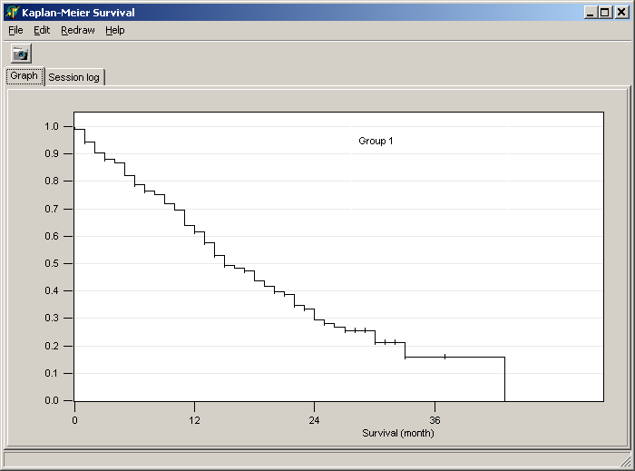
The example-graph shows Kaplan-Meier curves
for two sub-groups from the patient cohort (Group1
and Group2) which show clearly different
survival.
SUMO adds automatically a third group, which is generated
from all selected patients (Group1 + Group2 => Combined group).
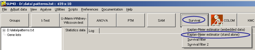
Click the Survival button and select Kaplan-Meier estimator (stand alone):
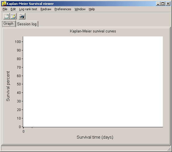
An empty Kaplan-Meier viewer opens up:
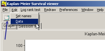
Select Main menu | Edit | Data or click the tool bar button to
open the integrated data editor.
A spreadsheet like form opens up:
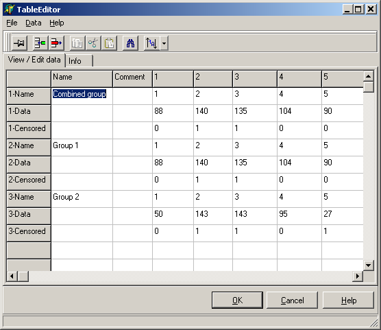
For each data set (=Kaplan-Meier curve) three data rows are found / required:
| x-Name | Name / ID for each single time point; may be empty |
| x-Data | Survival interval; a number (years or months or weeks
or days) giving the time interval until an individual died. required |
| x-Censored | Tag telling whether the individual died or was lost from the study (=Censored)
may be empty, i.e. all time points are uncensored. |
|
!! NB -- Changing order of rows (e.g. Censored /ID/Data) or missing single data rows will result in wrong or meaningless graphs. -- NB !! |
The columns contain:
| Column1=Name | Name of the dataset which will be shown in the graph May be empty |
| Column2=Comment | Any internal descriptive comment what the dataset
represents; May be empty |
| Other columns=1-xx | Data columns containing ID / survival / censoring data. If the Data field in the respective Data-row is empty or does not contain a number, the whole column for this particular data set will be ignored. |
You can freely edit values or Copy / Paste data from other sources.
In case your external data source contains data in a column oriented format
(i.e. survival data for the patients are in different rows), you may copy/paste
the respective data columns into the table.
When all required columns have been inserted, select
Main menu | Data | Transpose
to rotate the table (exchange columns with rows).
Take care that for each data set 3 rows are available in the correct order.
Also take care to have the two first columns containing dataset's name and
comment (or being empty).
In case the table is to small to accept all required columns/rows you can resize the table.
Select
Main menu | Data | Resize table
Click the Cancel button to close the form rejecting any modifications.
Click the OK button to use modified data.
Save the modified data set: Main Menu | File | Save as as tab-delimited text file
Reload a tab-delimited data file: Main menu | File | Open.
Export Kaplan-Meier curve data as tab-delimited file.
Select
Main menu | File | Export
For each single curve the file will contain:
Such a file may be imported into other drawing or spreadsheet programs.
Click into Series legend and drag legend with left-mouse-button pressed to a position you like,
The log rank test is the standard method to
compare two (or more) groups of survival analyses.
The log-rank test can be seen as censored data generalizations of linear rank
statistics such as the Wilcoxon rank sum test and Savage exponential score test. It is
also referred to as the generalized Savage test. It is also called Mantel-Cox test or
can be regarded as a time strtified Cochran-Mantel-Haenszel test.
The log-rank test is derived based on large-sample theory under the assumption
that the censoring distribution is independent of the failure distributions.
Log rank test only returns meaningful values if the Kaplan-Meier curves do
NOT intersect.
SUMO computes the Logrank test according to the method described in detail here:
The logrank test
J Martin Bland(1), Douglas G Altman(2)
1 Department of Health Sciences, University of York, York YO10 5DD,
2 Cancer Research UK/NHS Centre for Statistics in Medicine, Institute of Health Sciences, Oxford OX3 7LF
BMJ 2004;328:1073 (1 May), doi:10.1136/bmj.328.7447.1073
http://www.bmj.com/cgi/content/full/328/7447/1073
Select Main menu | Log rank test.
>An input dialog pops-up:
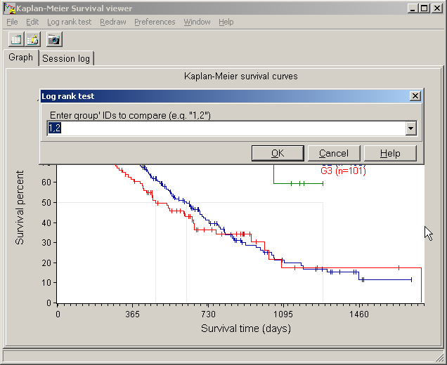
Define the numbers of the two groups to be tested (divided by semi colon), e.g. " 1,2 " to compare date from series 1 vs. series 2.
The Rresult is shown in a message box:
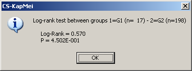
Additionally the numbers are copied to clipboard any may be pasted anywhere:
| Patient # Series 1 |
Patient # Series 2 |
Log rank test | p-value |
| 17 | 198 | 0.570 | 4.502E-001 |