Non parametric tests
A question in any kind of experimental data production is:
are my measured data only statistical noise from my measurement
system or are they statistically significant
Often this test is performed, assuming that
data are Gaussian like distributed around the "real" value. Under such an
assumption tests based on the well known Gaussian distribution may be
performed (e.g. t-test or ANOVA).
Here we can use two parameters (=> parametric tests), to exactly describe the
distribution: Mean and Standard deviation.
But often this assumption may not be true.
Under this assumption, more general non parametric tests not assuming a
specific distribution should be used.
SUMO offers two variants for non-parametric tests.
A. Tests which mainly analyze the position of the Median in the underlying data sets:
Man Whitney-, Wilcoxon-, Kruskal_Wallis- tests
B. Tests which analyze differences in both location and shape in the underlying data sets:
Kolmogorv-Smirnov Tests
1-class: U-/Man-Whitney test
2-class: U-/Man-Whitney test
2-class paired samples: Wilcoxon test
Multi-Class: Kruskal-Wallis test
How the tests work
One-class test
Two-class test
Assume an experiment with 2x3 hybs and following data for one gene:
| Un-treated |
Treated |
| 0.5 |
0.6 |
| 0.7 |
0.8 |
| 0.9 |
1.0 |
Join the data and sort (=rank) them by their ratio:
| Ratio: |
0.5 |
0.6 |
0.7 |
0.8 |
0.9 |
1.0 |
| Rank: |
1 |
2 |
3 |
4 |
5 |
6 |
Now calculate the rank sum for each group:
Un-treated: 1+3+5=9 =
R1>
Treated: 2+4+6=12 = R2
Question: How probable is it (p-value) to find a rank sum as small as 9 in the
data set.
Compute all possible rank sums:
1,2,3=6
1,2,4=7
1,2,5=8
1,2,6=9
1,3,4=8
1,3,5=9
1,3,6=10
1,4,5=10
1,4,6=11
1,5,6=12
2,3,4=9
2,3,5=10
2,3,6,=11
2,4,5=11
2,4,6=12
2,5,6=13
3,4,5=12
3,4,6=13
3,5,6=14
4,5,6=15
Total = 20 possible ranksums
For more then 3 groups ranksums are calculated accordingly
Build ranksum distribution:
| Rank sum |
6 |
7 |
8 |
9 |
10 |
11 |
12 |
13 |
14 |
15 |
| Number |
1 |
1 |
2 |
3 |
3 |
3 |
3 |
2 |
1 |
1 |
| p-value |
0.05 |
0.05 |
0.1 |
0.15 |
0.15 |
0.15 |
0.15 |
0.1 |
0.05 |
0.05 |
Now sum up the p-values for all rank sums below the
rank-sum of our smaller group (here: R1= 9)
=> p-value <=0.2 that the two groups are identical.
For larger groups it will become very time consuming to
calculate all possible rank sums. sumo calculates the correct rank sum
distribution up to a total group size of 32 (e.g. n1=16
hybs in one, n2=16 hybs in the other
group), which is done within a few seconds. For larger groups the rank sum
distribution is approximated by a Gaussian distribution deriving the p-value
from the Gauss distribution with:
| Normal approximation: |
z = ( U - mU) / sU
|
| Mean |
mU = n1 * n2/ 2
|
| Standard deviation: |
sU = sqrt (
( n1 * n2 * (n1 * n2 +1) ) / 12
) |
U1 = n1 * n2 +(n1 * ( n2 + 1)) / 2 - R1
U2 = n1 * n2 + (n1 * ( n2 + 1)) / 2 - R2
U = Min ( R1 , R2 )
Tie-correction
How to handle identical repeated measured values? Assume the following data set:
| Un-treated |
Treated |
| 0.5 |
0.7 |
| 0.7 |
0.9 |
| 0.9 |
1.1 |
Join the data and sort (=rank) them by their ratio:
| Ratio: |
0.5 |
0.7 |
0.7 |
0.9 |
0.9 |
1.1 |
| Rank': |
1 |
2 |
3 |
4 |
5 |
6 |
| Rank'': |
1 |
2 |
3 |
4 |
5 |
6 |
Obviously both rankings (Rank' and Rank'') are identical but would create different rank sums.
To avoid this for each run of repeated values (=Tie) the average rank for all
members of this run is calculated (=mid-rank) and used as tie-corrected rank:
| Ratio: |
0.5 |
0.7 |
0.7 |
0.9 |
0.9 |
1.1 |
| Rank: |
1 |
2.5 |
2.5 |
4.5 |
5.5 |
6 |
For more details about U-/Mann Whitney distribution go
here,
here or here.
A detailed description (German version) can be found at:
AG
Psychologische Methodenlehre, Uni Konstanz, compiled by Dr. Nagl, in this
document.
Single-class U-/Mann-Whitney-test
Here we want to test, whether a single gene is different to a fixed value (e.g. 0 regulation) in all selected hybridisations.
E.g. find genes which are highly regulated in all different cancer tissues => general impact for cancer.
A 1-class U-/Mann-Whitney test is not a "standard" statistical test, but we can perform it similarly like a 2-class test:
group 2 will contain only 1 member with ratio == 0.
All genes with low p-value are statistically significant regulated (i.e. either up- or down-regulated).
Click the Non-parametric tests button
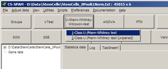
and select One-class U-/Mann-Whitney-Test
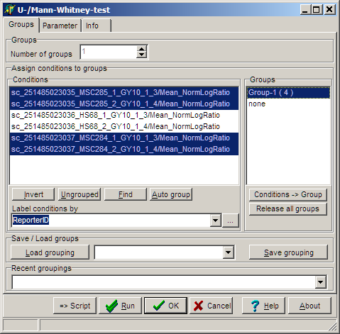
The parameter dialog-pops up
In the Groups tab-sheet select all required hybridisations:
On the Parameter page select:
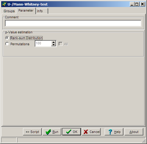
Select the algorithm how p-value is estimated:
- Ranksum-distribution to derive p-values from all possible rank sums which could arise from the
dataset.
- Permutations and number of permutations to estimate the p-value using a permutation scheme
Click OK button, and run the analysis.
In the experiment tree a new entry shows up:
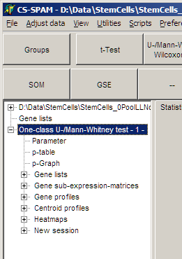
Like with t-tests (see above)
- View the Parameters for this analysis
- Use p-graph to select significant genesets
- Use Volano plot to select significant / reegulated gene sets
- View Profiles of selected genes
- View Centroid profilesfrom selected genes
- View Heat maps from selected genes
- ...
Save the matching genes:
- Gene lists: gene names and numerical test values
- Gene sub-expression matrices:
Expression matrix including gene-expression values
Two-class U-/Mann-Whitney-test
Here we test, whether a single gene is different in two selected sub-sets of our hybridisations (e.g. Cancer <=> Normal)
E.g. find genes which are clearly differentially regulated in the two sub-sets
(up<=>down or up<=>more up or down<=>more down).
All genes with low p-value are statistically significant regulated (i.e. either up- or down-regulated).
Click the Non-parametric tests button
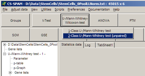
and select Two-class U-/Mann-Whitney-Test (unpaired)
Like above:
- Assign samples to groups
- Set parameters
- Set filters to selevt genes (p-graph/Volcano Plot
- View Profiles/Centroids/Heatmaps from selected genes
NB: Not very surprisingly you hardly get any any genes with low p-values when analysing small groups.
With e.g. 2 out of 6 you can only generate 15 different rank sums. Thus the smallest p-value will be 1/15~0.07.
Wilcoxon test (2-classpaired samples)
This test is used in situations in which the observations are paired: e.g. Blood pressure of patients before/after medicatuion.
This test assumes that there is information in the magnitudes of the differences
between paired observations, as well as the signs:
- Take the paired observations,
- Calculate the differences, and rank them from smallest to largest by ABSOLUTE value.
- Ignore values with difference=0
- Add all the ranks associated with positive differences, giving the T+ statistic.
- Add all the ranks associated with negative differences, giving the T- statistic.
- Finally, the P-value associated with this statistic is calculated the same way as for a standard U-/Man-Whitney test (see above).
Example: Assume measurement of a parameter for 10 individuals before and after treatment:
| Individual |
Before |
After |
Difference
(Before-After) |
|Difference| |
Raw Ranks
(one possibility, Ties!!) |
Ranks
Tie-corrected |
|
| 1 |
8 |
4 |
4 |
4 |
7 |
7.5 |
|
| 2 |
23 |
16 |
7 |
7 |
10 |
10 |
|
| 3 |
7 |
6 |
1 |
1 |
1 |
2 |
|
| 4 |
11 |
12 |
-1 |
1 |
2 |
2 |
|
| 5 |
5 |
6 |
-1 |
1 |
3 |
2 |
|
| 6 |
9 |
7 |
2 |
2 |
4 |
4.5 |
|
| 7 |
12 |
10 |
2 |
2 |
5 |
4.5 |
|
| 8 |
6 |
10 |
-4 |
4 |
8 |
7.5 |
|
| 9 |
10 |
10 |
0 |
0 |
- |
- |
|
| 10 |
18 |
13 |
5 |
5 |
9 |
9 |
|
| 11 |
9 |
6 |
3 |
3 |
6 |
6 |
|
Ranksum for negative values R-=2+2+7.5=11.5
Ranksum for positive values R+=2+4.5+4.5+6+7.5+9+10=435
NB: Tie correction: Ranke values for |Difference|=1 (3 concurrencies) can
not be defined. Therefore use average values for all three replicated values
(Ties). Here: For |Difference|=1 (1+2+3)/3=2; |Difference|=2 (4+5)/2=4.5;
|Difference|=4 (7+8)/2=7.5
Use ranksums R+=43.5,
N+=7 and R-=11.5,
N+=3 with normal 2-class U-Mann-Whitney
test (see above).
Multi-class Kruskal-Wallis
Here we test, whether a single gene is different between multiple (3 or more) selected sub-sets of our hybridisations (e.g.
Kidney <=> Liver <=> Lung <=> Heart)
E.g. find genes which are clearly different regulated in any different grouping
of the four sub-sets (K-LLH or L-KLH or KH-LL ...).
To do this SUMO builds all possible 2-group unique combinations of the sub set and performs for each combination a T-test. The lowest p-value of any of the possible combinations is reported as p-value for this gene.
All genes with low p-value are statistically significantly able to distinguish between the original sub-sets (in any way
described above).
Click the Non-parametric tests button
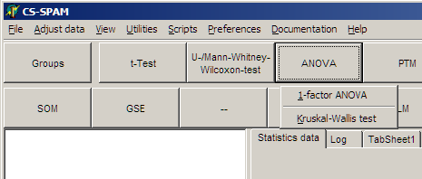
and select Kruskal-Wallis test
As already used:
- Assign groups, set parameters
- Filter significant genes
- Heatmaps, ... from selected genes
- ...
Wikipedia explains::
"... the Kolmogorov-Smirnov test (K-S test or KS test) is a nonparametric test of the equality of continuous, one-dimensional probability distributions that can be used to compare a sample with a reference probability distribution (one-sample K-S test), or to compare two samples (two-sample K-S test). ...
... The two-sample K-S test is one of the most useful and general nonparametric methods for comparing two samples, as it is sensitive to differences in both location and shape of the empirical cumulative distribution functions of the two samples. ..."
Build the "density function" from your data:
For our set of distinct measurements we build histograms counting the frequncies of measurements in intensity-/ratio bins.
- Convert the "density function" into the Empirical Distribution Function (EDF) of your data set (~cumulative density function):
- find the position with largest difference Dn,m between the two distributions.
- Derive a p-value from Dn,m with samplesizes (n for first data set and m for second dataset) as parameters.
Following Wikipedia we would reject the
null hypothesis at level α if:
(1)
with
(2)
Inserting (2) in (1) and performing some algebraic transformations we can compute α depending on Dn,mwith parameters n and m:
This α is the p-value (depending on Dn,m, n, m) at which we would reject the null hypotheses.
Click the Non-parametric tests button
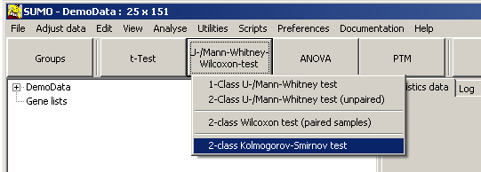
and select Kolmogorov-Smirnov-test.
As already used:
- Assign groups, set parameters
- Filter significant genes
- Heatmaps, ... from selected genes
- ...
To explore in more details the KS-Test - with demo data or custom datasets - see Utilities | Statistics test | Kolmogorov-Smirnov test.
As described above, used to test similarity between two groups of data.
Multi-class Kolmogorov-Smirnov test
The Kolmogorov-Smirnov test is defined to compare 2 data groups.
But similar to the Multi-class t-test we can perform a multi-class Kolmogorov-Smirnov test.
For all possible unique combinatons of two groups (e.g. Group1 vs Group2, 1 vs 3,..,2 vs 3,...(n-1) vs n, but not 2 vs 1,...) we perform a Kolmogorov-Smirnov test and memorize all respective p-values.
Under the null-hypothesis (all groups are randomly distributed), thus all pairwise tests should report a p ~ 1.
If one or more group pairs have different distributions for one feature, one or mores p-values will be p << 1
And those are the features which may be helpful to explain the grouping.
On the Paramter-tabsheet you may chosse:
- MIN p-value between any group-pair
E.g. you defined 5 groups =>10 group pairs to test.
As long as at least ONE pair delivers a p-value<=Threshold, this feature will be reported as signifcant.
A filter strategy comparable to ANOVA
- MAX p-value between any group-pair
E.g. you defined 5 groups =>10 group pairs.
This time we require that ALL 10 pairs deliver a p-value<=Threshold, to filter this feature as signifcant
And thus even the largest p-value of from any of the pairs must be <=Threshold.
A filter, much more restrictive compared to ANOVA, and returning a different kind of information.